Analysis:

Functions in this module perform analysis on data and output interpretable results.

Example functions include calculating firing rate, successrate, direction tuning, dimensionality, among others.

API

The analysis module is broken up into the following submodules. The functions and classes within base, behavior, celltype, tuning, and kfdecoder are accessible directly from aopy.analysis. Additional submodules can be accessed with the appropriate aopy.analysis.<submodule> import.

Base

aopy.analysis.base.align_spatial_maps(data1, data2)

Align two input maps by finding the location of the peak of the 2D correlation function. Note, if these shifts are unexpectedly high, there is likely not high enough correlation between the maps and the alignment should not be used. This function replaces input NaN values with 0 and uses 0-padding for all edge conditions.

Parameters:

• data1 (nrow, ncol) – First input data array, used as baseline map.

• data2 (nrow, ncol) – Second input data array, will be shifted to match the baseline map.

Returns:

tuple containing:

data2_align (nrow, ncol): aligned version of data2

shifts (tuple): contains (row_shifts, col_shifts)

Return type:

tuple

aopy.analysis.base.calc_ISI(data, fs, bin_width, hist_width, plot_flag=False)

Computes inter-spike interval histogram. The input data is the sampled thresholded data (0 or 1 data).

Example

>>> data = np.array([[0, 1, 0, 0, 1, 0, 0, 1, 0, 1, 0, 1, 1, 1, 0, 0, 0, 1],[1, 1, 1, 0, 0, 0, 1, 0, 0, 1, 0, 0, 0, 1, 1, 0, 1, 0]])
>>> data_T = data.T
>>> fs = 100
>>> bin_width = 0.01
>>> hist_width = 0.1
>>> ISI_hist, hist_bins = analysis.calc_ISI(data_T, fs, bin_width, hist_width)
>>> print(ISI_hist)
    [[0. 0.]
    [2. 3.]
    [2. 1.]
    [2. 1.]
    [1. 2.]
    [0. 0.]
    [0. 0.]
    [0. 0.]
    [0. 0.]]

Parameters:

• data (nt, n_unit) – time series spike data with multiple units.

• fs (float) – sampling rate of data [Hz]

• bin_width (float) – bin_width to compute histogram [s]

• hist_width (float) – determines bin edge (0 < t < histo_width) [s]

• plot_flag (bool, optional) – display histogram. In plotting, number of intervals is summed across units.

Returns:

tuple containing:

ISI_hist (n_bins, n_unit): number of intervals

hist_bins (n_bins): bin edge to compute histogram

Return type:

tuple

aopy.analysis.base.calc_confidence_interval_overlap(CI1, CI2)

Calculate the overlap between two confidence intervals.

Parameters:

• CI1 (tuple or list) – Tuple containing the lower and upper bounds of the first confidence interval.

• CI2 (tuple or list) – Tuple containing the lower and upper bounds of the second confidence interval.

Returns:

Overlap ratio (0 to 1) between the two confidence intervals.

Return type:

(float)

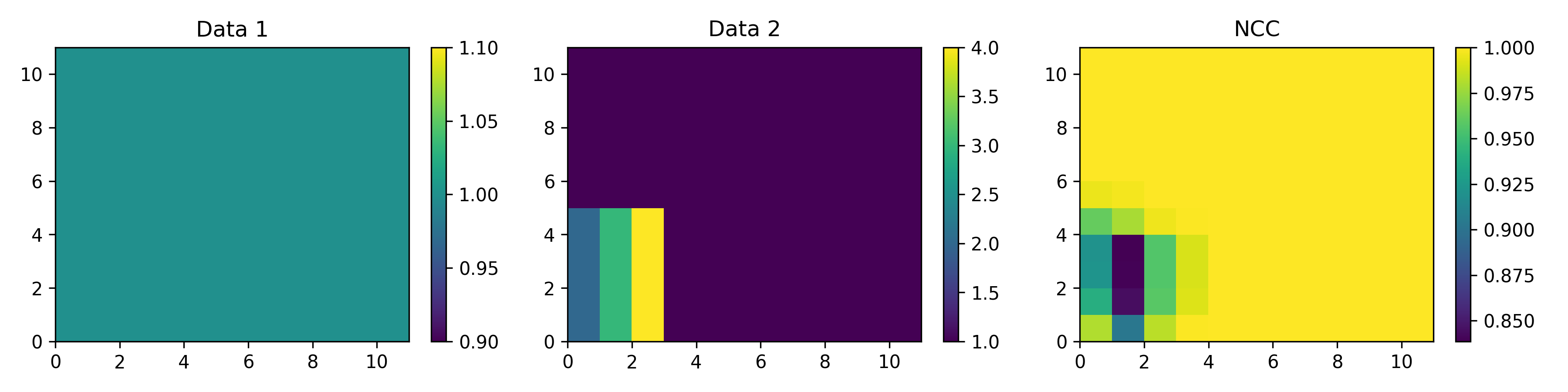
aopy.analysis.base.calc_corr2_map(data1, data2, knlsz=15, align_maps=False)

This function creates a map showning the local correlation between two input datamaps. If specified, it also aligns the input maps by finding the location of the peak of the 2D correlation function. Note, if these shifts are unexpectedly high, there is likely not high enough correlation between the datamaps and alignment should not be used. This function uses 0-padding for all edge conditions and replaces input NaN values with 0 to calculate the correlation map. After the correlation map is calculated, all values were NaN in the input data are again set to NaN. If a window of data has all 0’s, the NCC is set to nan. Note, the worst correlation in the example image is not at the edge of the image because of zero padding.

Parameters:

• data1 (nrow, ncol) – First input data array. Used as baseline if map alignment is required.

• data2 (nrow, ncol) – Second input data array. Shifted to match the baseline if map alignment is required

• knlsz (int) – Length of the kernel window in units of data points. The kernel is a square so each side will have the lenght specified here. This value should always be odd.

• align_maps (bool) – Whether or not to align maps.

Returns:

Tuple containing:

NCC (nrow, ncol): Spatial correlation map (NCC: normalized correlatoin coefficient)

shifts (tuple): Contains (row_shifts, col_shifts)

Return type:

tuple

aopy.analysis.base.calc_corr_over_elec_distance(elec_data, elec_pos, bins=20, method='spearman', exclude_zero_dist=True)

Calculates mean absolute correlation between acq_data across channels with the same distance between them.

Parameters:

• elec_data (nt, nelec) – electrode data with nch corresponding to elec_pos

• elec_pos (nelec, 2) – x, y position of each electrode

• bins (int or array) – input into scipy.stats.binned_statistic, can be a number or a set of bins

• method (str, optional) – correlation method to use (‘pearson’ or ‘spearman’)

• exclude_zero_dist (bool, optional) – whether to exclude distances that are equal to zero. default True

Returns:

tuple containing:

dist (nbins): electrode distance at each bin

corr (nbins): correlation at each bin

Return type:

tuple

Updated:

2024-03-13 (LRS): Changed input from acq_data and acq_ch to elec_data.

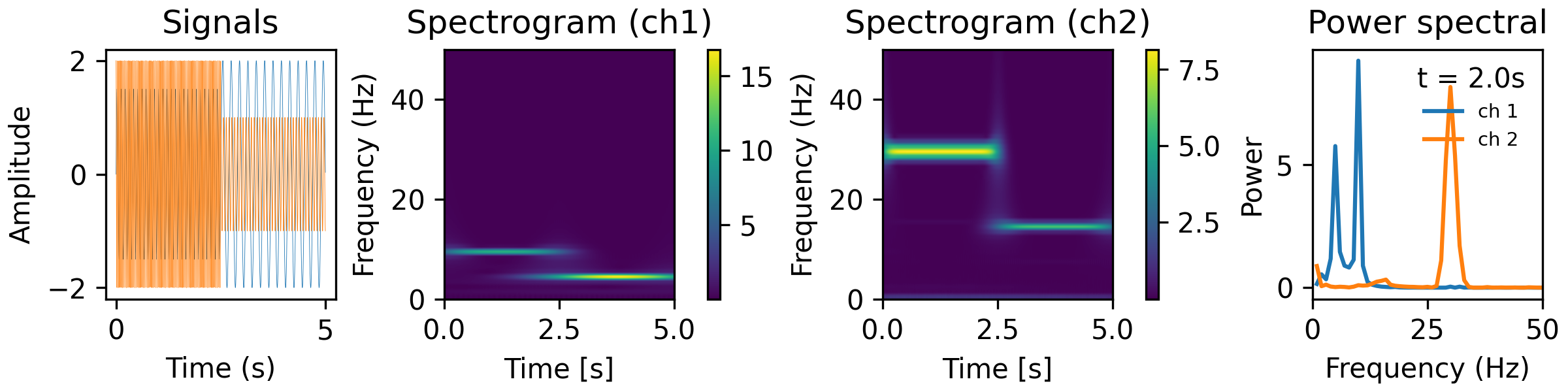
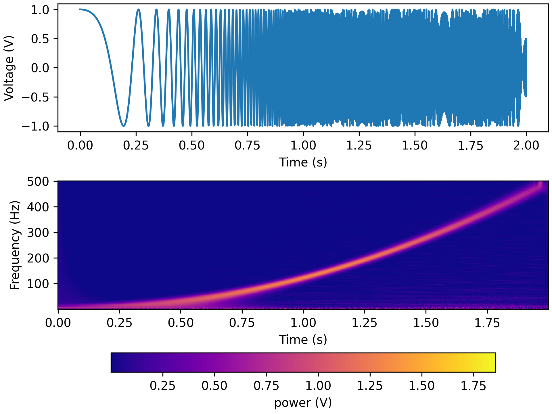
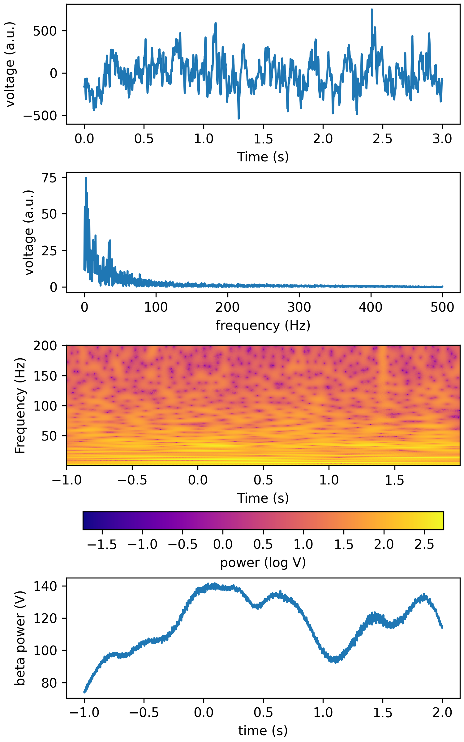
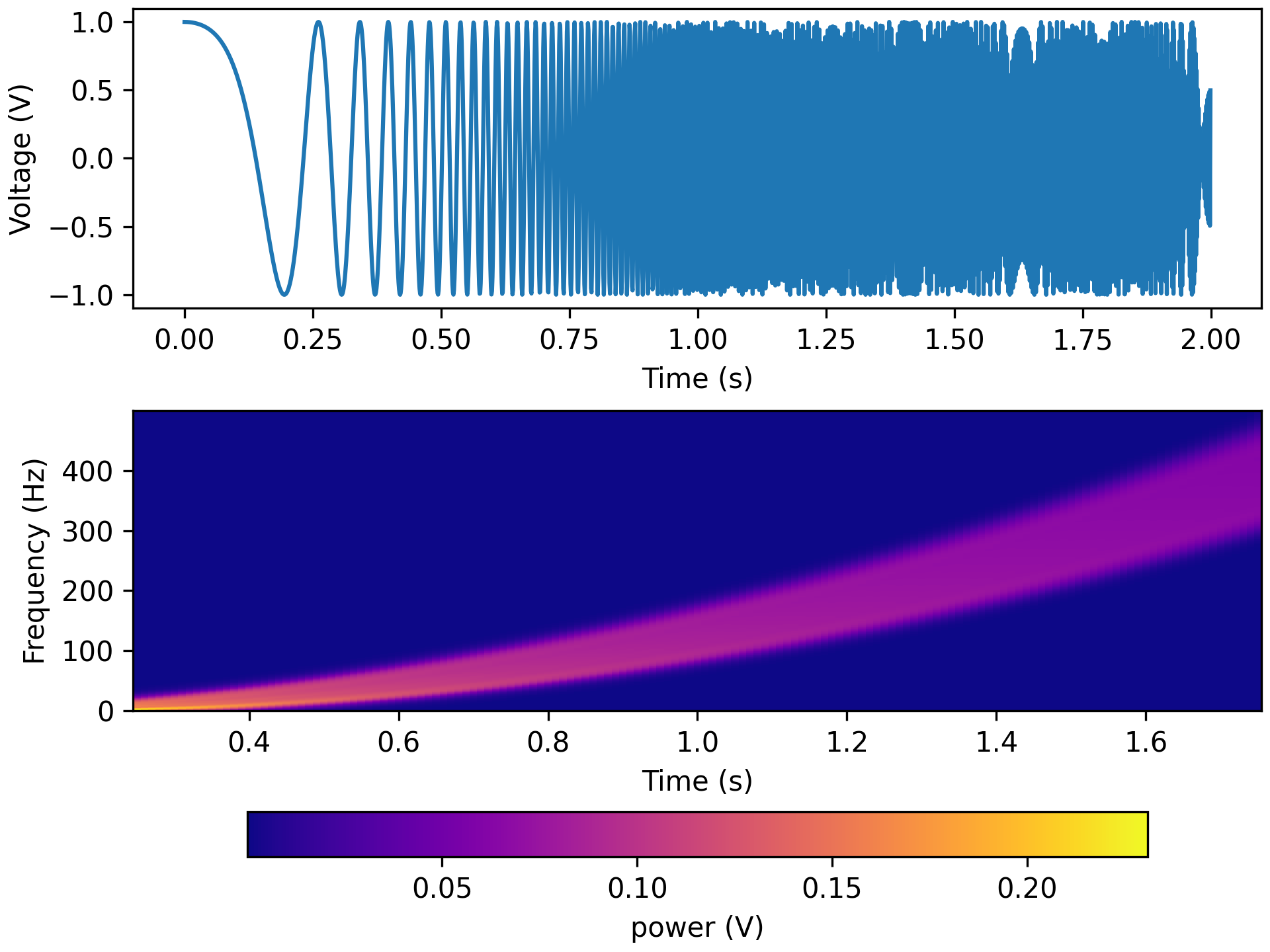
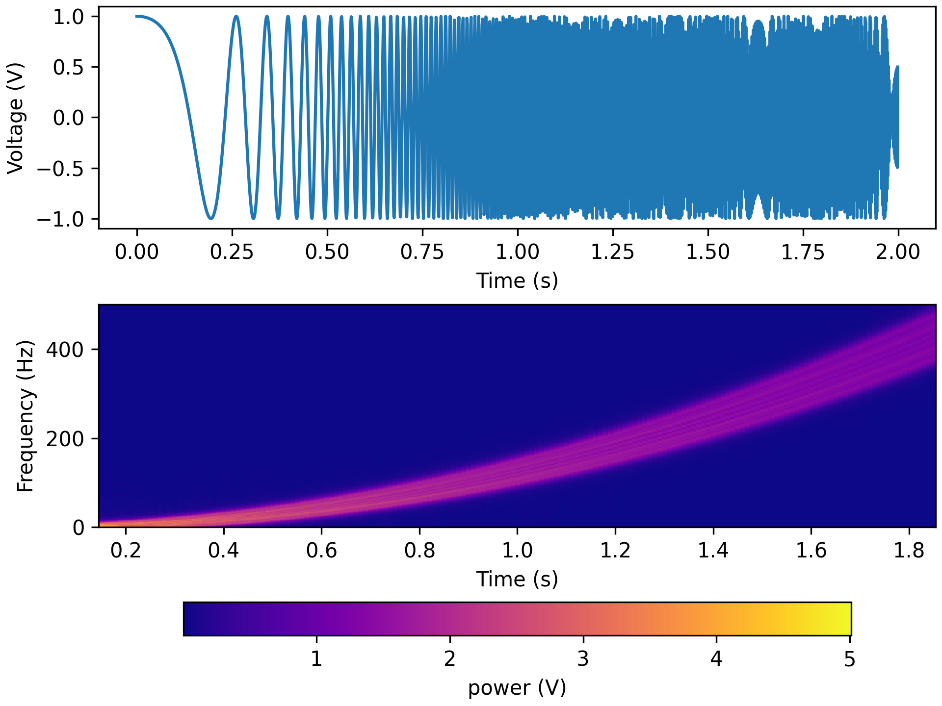
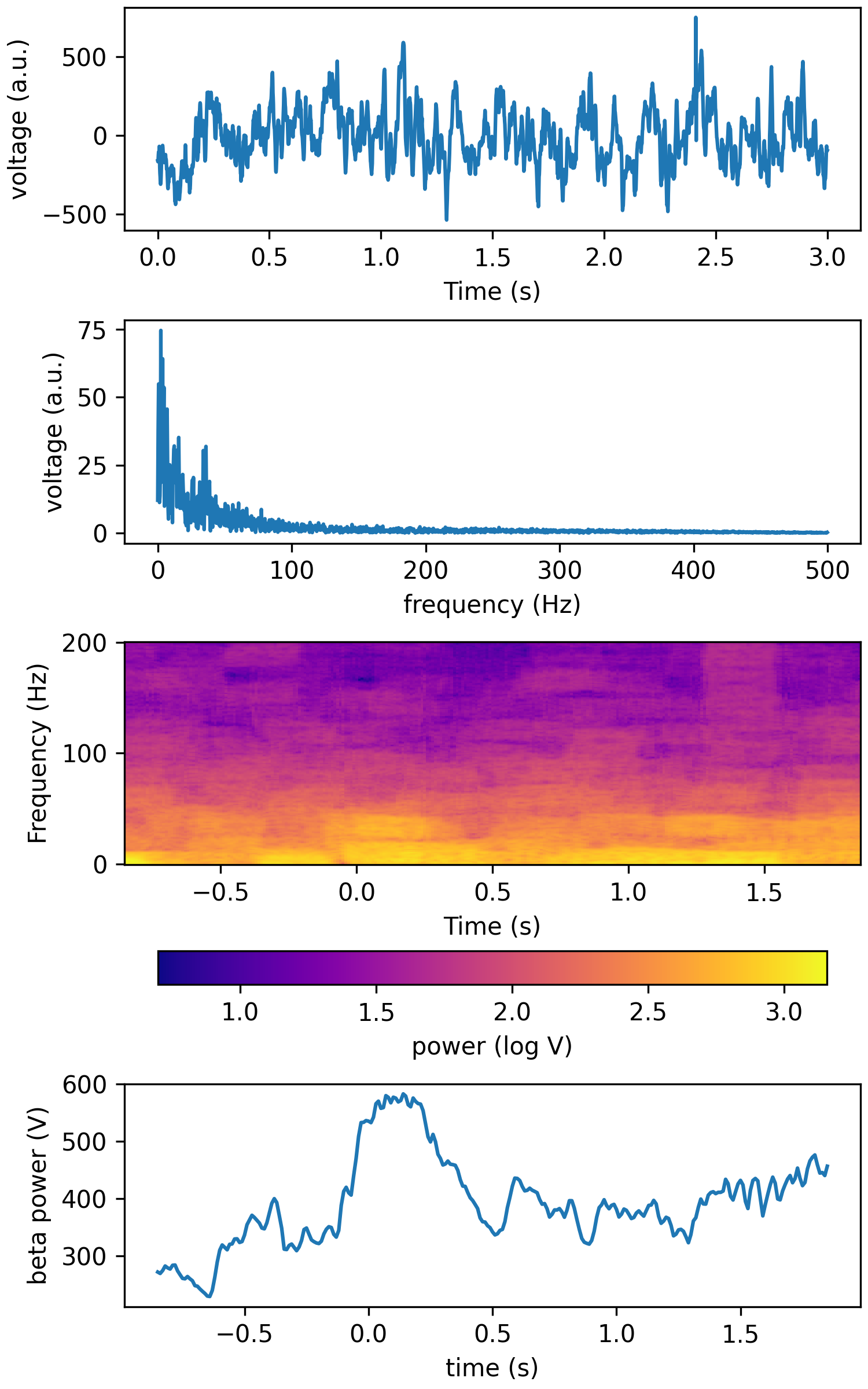
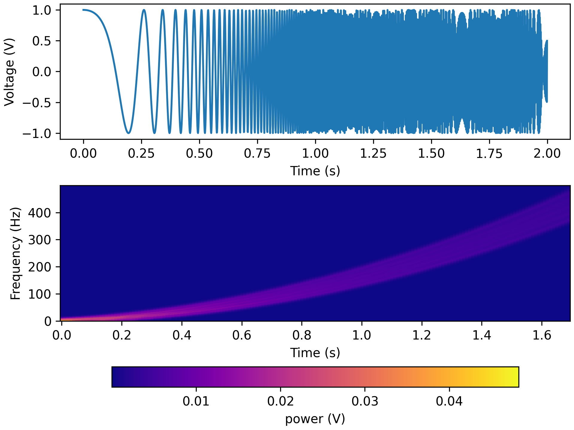
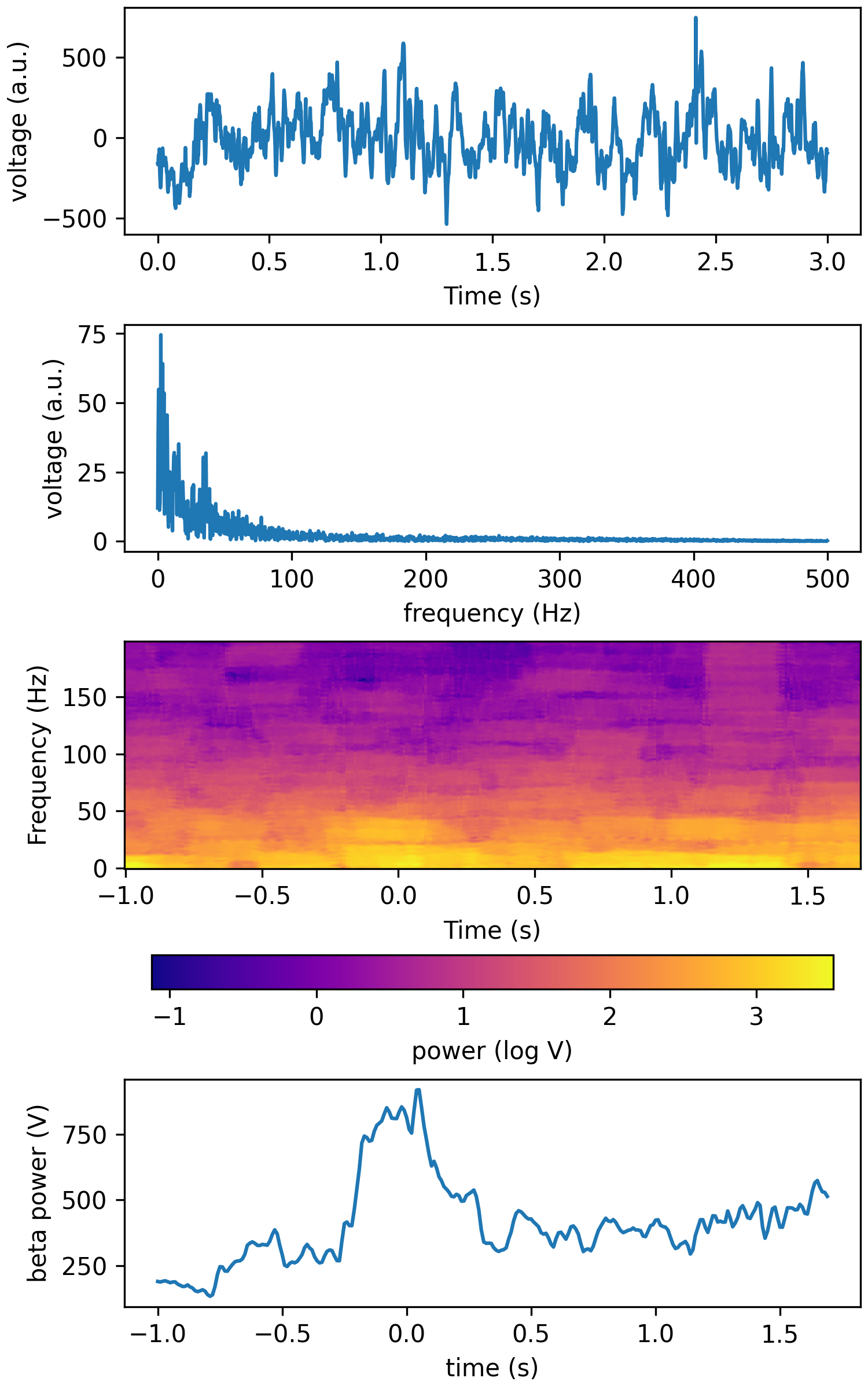
aopy.analysis.base.calc_cwt_tfr(data, freqs, samplerate, fb=1.5, f0_norm=1.0, method='fft', complex_output=False, verbose=False)

Use morlet wavelet decomposition to calculate a time-frequency representation of your data.

Parameters:

• data (nt, nch) – time series data

• freqs (nfreq) – frequencies to decompose

• samplerate (float) – sampling rate of the data

• fb (float, optional) – time-decay parameter, inverse relationship with bandwidth of the wavelets; setting a higher number results in narrower frequency resolution

• f0_norm (float, optional) – center frequency of the wavelets, normalized to the sampling rate. Default to 1.0, or the same frequency as the sampling rate.

• method (str, optional) – either ‘fft’, or ‘conv’, which can be faster for shorter data. Defaults to ‘fft’.

• complex_output (bool, optional) – output complex output or magnitdue. Default False.

• verbose (bool, optional) – print out information about the wavelets

Returns:

tuple containing:

freqs (nfreq): frequency axis in Hz

time (nt): time axis in seconds

spec (nfreq, nt, nch): tfr representation for each channel

Return type:

tuple

Examples

from analyze/tests/analysis_tests import HelperFunctions
fb = 10.
f0_norm = 2.
freqs = np.linspace(1,50,50)
tfr_fun = lambda data, fs: aopy.analysis.calc_cwt_tfr(data, freqs, fs, fb=fb, f0_norm=f0_norm, verbose=True)
HelperFunctions.test_tfr_sines(tfr_fun)

freqs = np.linspace(1,500,500)
tfr_fun = lambda data, fs: aopy.analysis.calc_cwt_tfr(data, freqs, fs, fb=fb, f0_norm=f0_norm, verbose=True)
HelperFunctions.test_tfr_chirp(tfr_fun)

freqs = np.linspace(1,200,200)
tfr_fun = lambda data, fs: aopy.analysis.calc_cwt_tfr(data, freqs, fs, fb=fb, f0_norm=f0_norm, verbose=True)
HelperFunctions.test_tfr_lfp(tfr_fun)

aopy.analysis.base.calc_erp(data, event_times, time_before, time_after, samplerate, subtract_baseline=True, baseline_window=None)

Calculates the event-related potential (ERP) for the given timeseries data.

Parameters:

• data (nt, nch) – timeseries data across channels

• event_times (ntrial) – list of event times

• time_before (float) – number of seconds to include before each event

• time_after (float) – number of seconds to include after each event

• samplerate (float) – sampling rate of the data

• subtract_baseline (bool, optional) – if True, subtract the mean of the aligned data during the time_before period preceding each event (using nanmean). Must supply a positive time_before. Default True

• baseline_window ((2,) float, optional) – range of time to compute baseline (in seconds before event) Default is the entire time_before period.

Returns:

array of event-aligned responses for each channel during the given time periods

Return type:

(nt, nch, ntr)

aopy.analysis.base.calc_fdrc_ranktest(altdata, nulldata_dist, alternative='greater', nan_policy='raise', alpha=0.05)

Compute statistical significance using the Wilcoxon signed-rank test with FDR correction.

Parameters:

• altdata (nch) – Observed data values.

• nulldata_dist (n_null, nch) – Null distribution for comparison.

• alternative (str, optional) – Hypothesis test alternative (‘greater’, ‘less’, ‘two-sided’). Defaults to ‘greater’.

• nan_policy (str, optional) – Handling of NaN values. Defaults to ‘raise’.

• alpha (float, optional) – Significance level. Defaults to 0.05.

Returns:

tuple containing:

effect_size (nch): differences between the alternative and null data

p_fdrc (nch): Adjusted p-values for each alternative hypothesis test.

Return type:

tuple

aopy.analysis.base.calc_freq_domain_amplitude(data, samplerate, rms=False)

Use FFT to decompose time series data into frequency domain to calculate the amplitude of the non-negative frequency components

Parameters:

• data (nt, nch) – timeseries data, can be a single channel vector

• samplerate (float) – sampling rate of the data

• rms (bool, optional) – compute root-mean square amplitude instead of peak amplitude

Returns:

Tuple containing:

freqs (nt/2): array of frequencies (essentially the x axis of a spectrogram)

amplitudes (nt/2, nch): array of amplitudes at the above frequencies (the y axis)

Return type:

tuple

aopy.analysis.base.calc_freq_domain_values(data, samplerate)

Use FFT to decompose time series data into frequency domain and return non-negative frequency components For math details, see: https://www.sjsu.edu/people/burford.furman/docs/me120/FFT_tutorial_NI.pdf

Parameters:

• data (nt, nch) – timeseries data, can be a single channel vector

• samplerate (float) – sampling rate of the data

Returns:

Tuple containing:

freqs (nt/2): array of frequencies (essentially the x axis of a spectrogram)

freqvalues (nt/2, nch): array of complex numbers at the above frequencies (each containing magnitude and phase)

Return type:

tuple

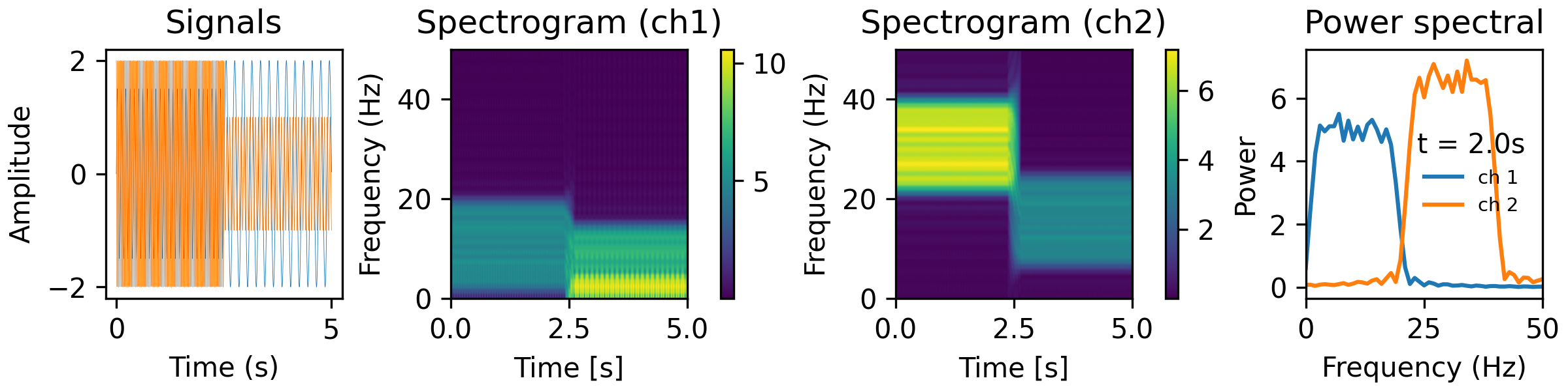
aopy.analysis.base.calc_ft_tfr(data, samplerate, win_t, step, f_max=None, pad=2, window=None, detrend='constant', complex_output=False)

Short-time fourier transform. Makes use of scipy.signal.spectrogram to compute a fast spectrogram.

Parameters:

• data (nt, nch) – timeseries data.

• samplerate (float) – sampling rate of the data.

• win_t (float) – window size in seconds.

• step (float) – step size in seconds.

• f_max (float) – frequency range to return in Hz ([0, f_max]). Defaults to samplerate/2.

• pad (int) – padding factor for the FFT. This should be 1 or a multiple of 2. For N=500, if pad=1, we pad the FFT to 512 points. If pad=2, we pad the FFT to 1024 points. If pad=4, we pad the FFT to 2024 points.

• window (tuple, optional) – see scipy documentation. Defaults to None.

• detrend (str, optional) – see scipy documentation. Defaults to ‘constant’.

• complex_output (bool) – if True, return the complex signal instead of magnitude. Default False.

Returns:

Tuple containing:

f (n_freq): frequency axis for spectrogram

t (n_time): time axis for spectrogram

spec (n_freq,n_time,nch): multitaper spectrogram estimate

Return type:

tuple

Examples

from analyze/tests/analysis_tests import HelperFunctions
win_t = 0.5
step = 0.01
f_max = 50
tfr_fun = lambda data, fs: aopy.analysis.calc_ft_tfr(data, fs, win_t, step, f_max, pad=3, window=('tukey', 0.5))
HelperFunctions.test_tfr_sines(tfr_fun)

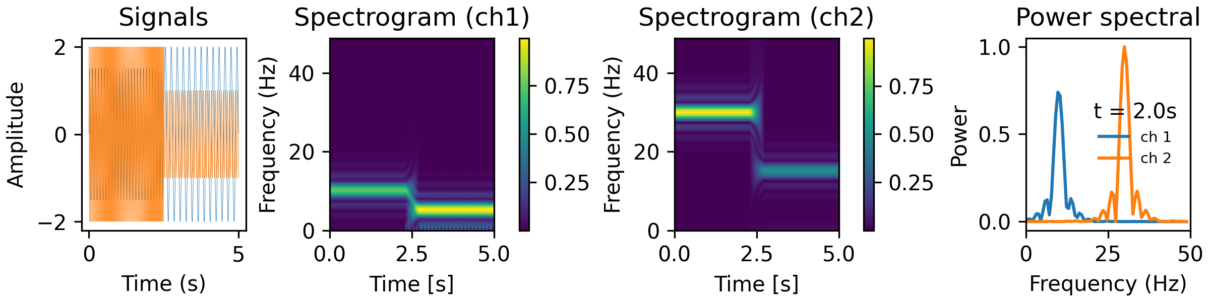
f_max = 500
tfr_fun = lambda data, fs: aopy.analysis.calc_ft_tfr(data, fs, win_t, step, f_max, pad=3, window=('tukey', 0.5))
HelperFunctions.test_tfr_chirp(tfr_fun)

f_max = 200
tfr_fun = lambda data, fs: aopy.analysis.calc_ft_tfr(data, fs, win_t, step, f_max, pad=3, window=('tukey', 0.5))
HelperFunctions.test_tfr_lfp(tfr_fun)

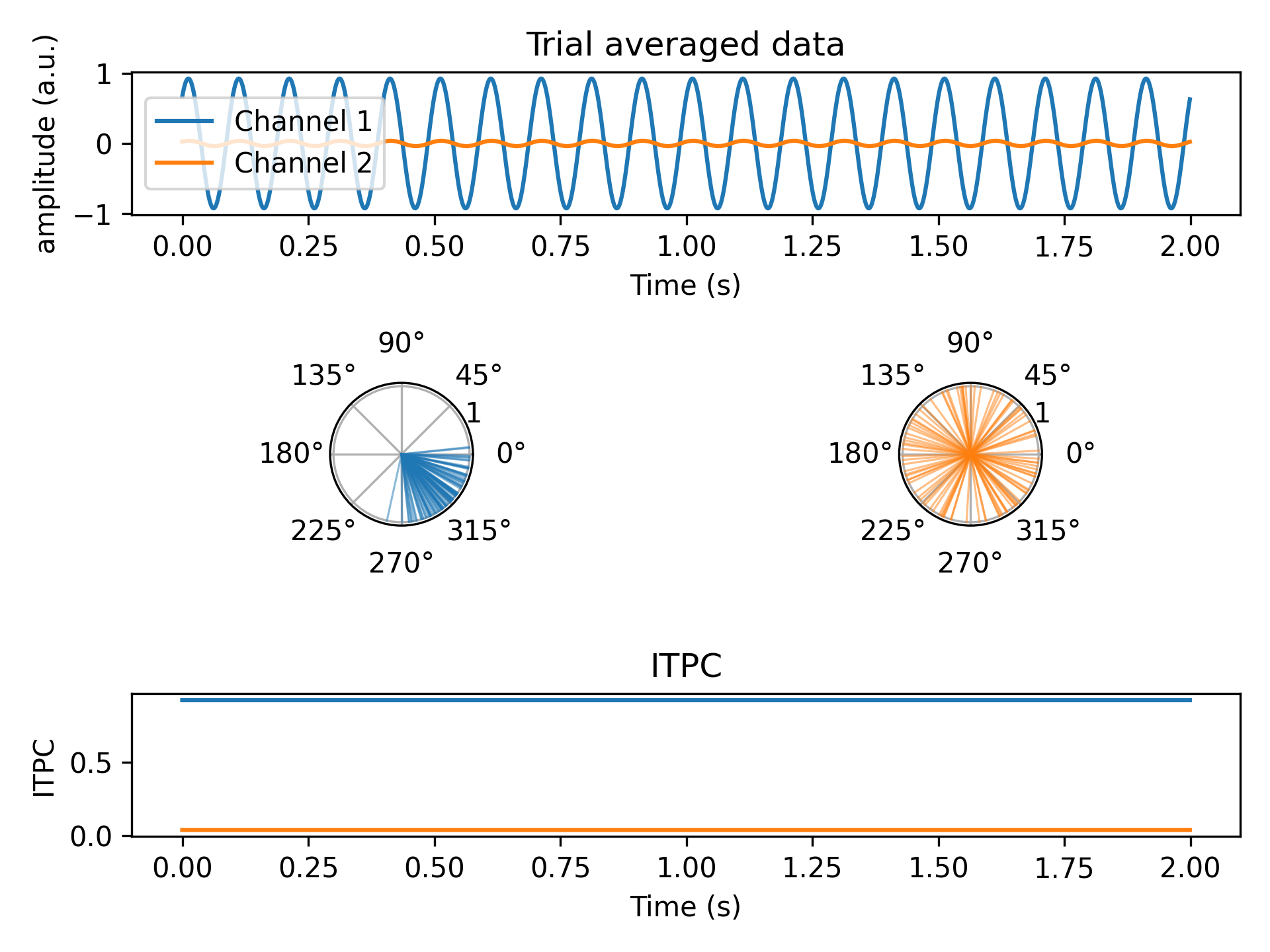
aopy.analysis.base.calc_itpc(analytical_signals)

Computes inter-trial phase clustering (ITPC) from analytical signals of evoked potentials. ITPC is computed as the magnitude of the mean of the complex signal across trials at each timepoint (think vector average). This captures the similarity of phases across trials. ITPC ranges from 0 to 1, where 0 indicates uniformly random phases and 1 indicates perfect phase alignment.

From Cohen, M. X. (2014). Analyzing neural time series data: theory and practice. MIT press.

\[ITPC = \frac{1}{N} |\sum_{k=1}^{N} e^{i\theta_k}|\]

Parameters:

analytical_signals (nt, nch, ntr) – analytical signal of the evoked potential (np.complex128)

Returns:

itpc values for each channel (ranges from 0 to 1)

Return type:

(nt, nch)

Examples

Generate two channels of data with different phase distributions across trials

fs = 1000
nt = fs * 2
ntr = 100
t = np.arange(nt)/fs
data = np.zeros((t.shape[0],2,ntr)) # 2 channels

# 10 Hz sine with gaussian phase distribution across trials
for tr in range(ntr):
    data[:,0,tr] = np.sin(2*np.pi*10*t + np.random.normal(np.pi/4, np.pi/8))

# 10 Hz sine with uniform random phase distribution across trials
for tr in range(ntr):
    data[:,1,tr] = np.sin(2*np.pi*10*t + np.random.uniform(-np.pi, np.pi))

Calculate an analytical signal using hilbert transform, then apply ITPC

im_data = signal.hilbert(data, axis=0)
itpc = aopy.analysis.calc_itpc(im_data)

plt.figure()

# Plot the data
plt.subplot(3,1,1)
aopy.visualization.plot_timeseries(np.mean(data, axis=2), fs)
plt.legend(['Channel 1', 'Channel 2'])
plt.ylabel('amplitude (a.u.)')
plt.title('Trial averaged data')

# Plot the angles at the first timepoint
angles = np.angle(im_data[0])
plt.subplot(3,2,3, projection= 'polar')
aopy.visualization.plot_angles(angles[0,:], color='tab:blue', alpha=0.5, linewidth=0.75)
plt.subplot(3,2,4, projection= 'polar')
aopy.visualization.plot_angles(angles[1,:], color='tab:orange', alpha=0.5, linewidth=0.75)

# Plot ITPC
plt.subplot(3,1,3)
aopy.visualization.plot_timeseries(itpc, fs)
plt.ylabel('ITPC')
plt.title('ITPC')

aopy.analysis.base.calc_max_erp(data, event_times, time_before, time_after, samplerate, subtract_baseline=True, baseline_window=None, max_search_window=None, trial_average=True)

Calculates the maximum (across time) mean (across trials) event-related potential (ERP) for the given timeseries data. Identical to get_max_erp() except this function takes timeseries data. If you already have trial-aligned erp (e.g. from calc_erp(), then use get_max_erp() instead.

Parameters:

• data (nt, nch) – timeseries data across channels

• event_times (ntrial) – list of event times

• time_before (float) – number of seconds to include before each event

• time_after (float) – number of seconds to include after each event

• samplerate (float) – sampling rate of the data

• subtract_baseline (bool, optional) – if True, subtract the mean of the aligned data during the time_before period preceding each event. Must supply a positive time_before. Default True

• baseline_window ((2,) float, optional) – range of time to compute baseline (in seconds before event) Default is the entire time_before period.

• max_search_window ((2,) float, optional) – range of time to search for maximum value (in seconds after event). Default is the entire time_after period.

• trial_average (bool, optional) – by default, average across trials before calculating max

Returns:

array of maximum mean-ERP for each channel during the given time periods

Return type:

nch

aopy.analysis.base.calc_mt_psd(data, fs, bw=None, nfft=None, adaptive=False, jackknife=True, sides='default')

Computes power spectral density using Multitaper functions from nitime.

Parameters:

• data (nt, nch) – time series data where time axis is assumed to be on the last axis

• fs (float) – sampling rate of the signal

• bw (float) – sampling bandwidth of the data tapers in Hz

• adaptive (bool) – Use an adaptive weighting routine to combine the PSD estimates of different tapers.

• jackknife (bool) – Use the jackknife method to make an estimate of the PSD variance at each point.

• sides (str) – This determines which sides of the spectrum to return.

Returns:

Tuple containing:

f (nfft): Frequency points vector

psd_est (nfft, nch): estimated power spectral density (PSD)

nu (nfft, nch): if jackknife = True; estimated variance of the log-psd. If Jackknife = False; degrees of freedom in a chi square model of how the estimated psd is distributed wrt true log - PSD

Return type:

tuple

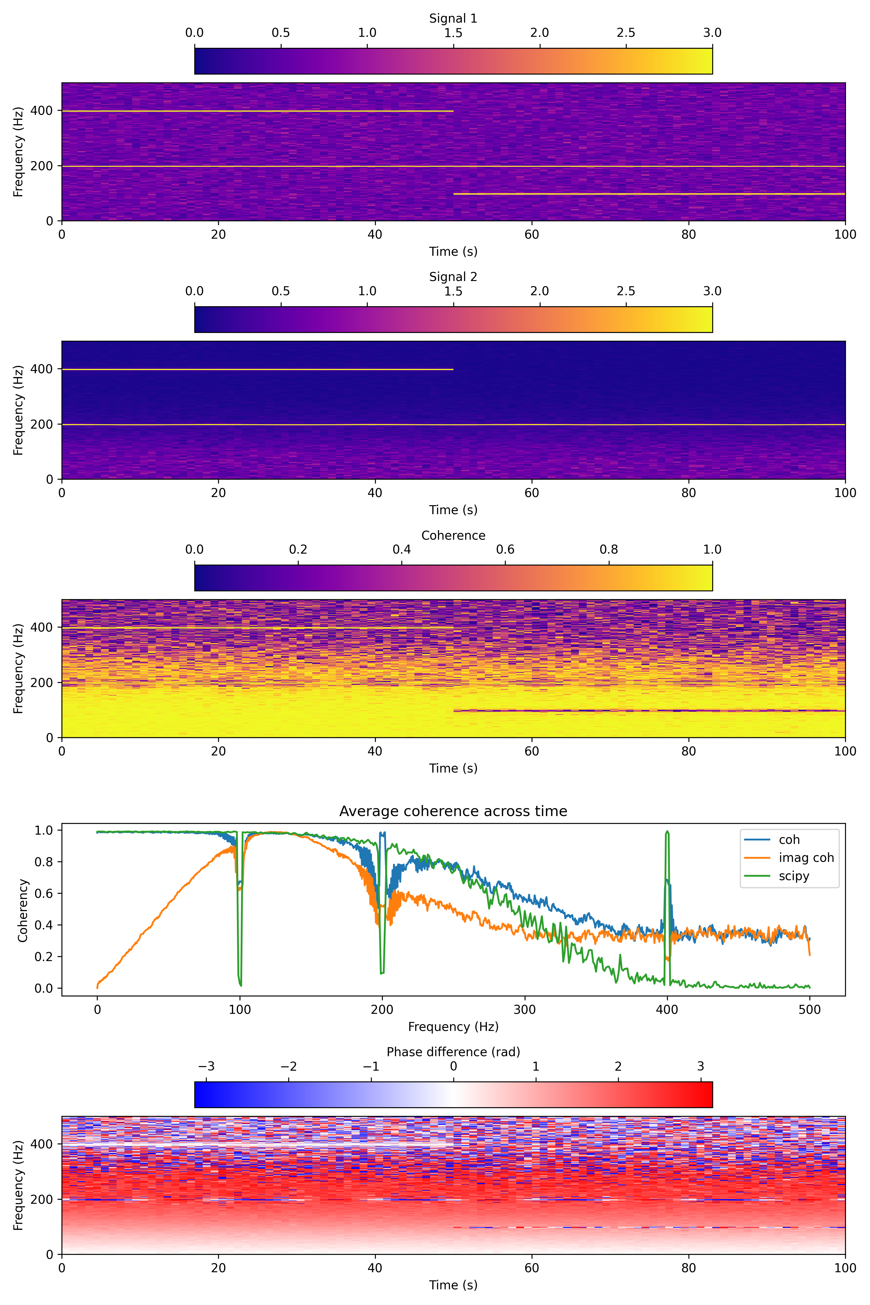
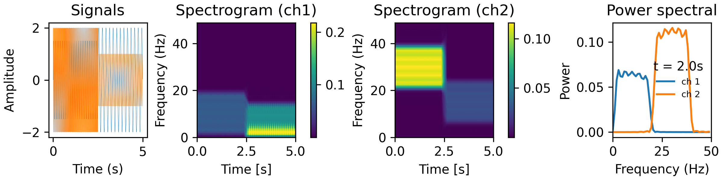
aopy.analysis.base.calc_mt_tfcoh(data, ch, n, p, k, fs, step, fk=None, pad=2, ref=False, imaginary=False, return_angle=False, dtype='float64', workers=None)

Computes moving window time-frequency coherence averaged across trials between selected channels. This is loosely based on pesaran lab code, modified to be more compatible with calc_mt_tfr(). The coherence computations are from https://doi.org/10.7551/mitpress/9609.001.0001

Given analytical signals Xk1 and Xk2, coherence is computed as:

# Compute power and cross-spectral power
S1 = np.sum(Xk*Xk.conj(), axis=1) # sum across tapers and trials
S2 = np.sum(Yk*Yk.conj(), axis=1) # sum across tapers and trials
S12 = np.sum(Xk*Yk.conj(), axis=1) # sum across tapers and trials

# Coherence
coh = np.abs(S12/np.sqrt(S1*S2))**2

# Imaginary coherence
coh = np.abs(np.imag(S12/np.sqrt(S1*S2)))

Parameters:

• data ((nt,nch,ntr) array) – evoked potential across all channels and trials

• ch ((2,) tuple) – the two channel indices between which coherence will be computed

• n (float) – window length in seconds

• p (float) – standardized half bandwidth in hz

• k (int) – number of DPSS tapers to use

• fs (float) – sampling rate in Hz.

• step (float) – window step size in seconds.

• fk (float, optional) – frequency range to return in Hz ([0, fk]). Default is fs/2.

• pad (int, optional) – padding factor for the FFT. This should be 1 or a multiple of 2. For nt=500, if pad=1, we pad the FFT to 512 points. If pad=2, we pad the FFT to 1024 points. If pad=4, we pad the FFT to 2024 points. Default is 2.

• ref (bool, optional) – referencing flag. If True, mean of neural signals across electrodes for each time window is subtracted to remove common noise so that You can get spacially-localized signals. If you only analyze single channel data, this has to be False. This paper discuss referencing scheme https://iopscience.iop.org/article/10.1088/1741-2552/abce3c Default is False.

• imaginary (bool, optional) – if True, compute imaginary coherence.

• return_angle (bool, optional) – if True, also return the phase difference between the two channels. For example if ch = [ch1, ch0], angles correspond to phase differences from ch1 to ch0 (i.e. angle ≈ phase(ch1) - phase(ch0)). Default is False.

• dtype (str, optional) – dtype of the output. Default ‘float64’

• workers (int, optional) – Number of workers argument to pass to scipy.fft.fft. Default None.

Returns:

tuple containing:

f (n_freq): frequency axis

t (n_time): time axis

coh (n_freq,n_time): magnitude squared coherence or imaginary coherence (0 <= coh <= 1)

angle (n_freq,n_time): phase difference between the two channels in radians (optional output, -pi <= angle <= pi)

Return type:

tuple

See also

calc_mt_tfr()

Examples

fs = 1000
N = 1e5
T = N/fs
amp = 20
noise_power = 0.001 * fs / 2
time = np.arange(N) / fs

Generate two test signals with common low-frequency signals, except at a given freq (100 Hz)

rng = np.random.default_rng(seed=0)
signal1 = rng.normal(scale=np.sqrt(noise_power), size=time.shape)

b, a = scipy.signal.butter(2, 0.25, 'low')
signal2 = scipy.signal.lfilter(b, a, signal1)
signal2 += rng.normal(scale=0.1*np.sqrt(noise_power), size=time.shape)

# Add a 100 hz sine wave only to signal 1
freq = 100.0
signal1[time > T/2] += amp*np.sin(2*np.pi*freq*time[time > T/2])

# Add a 400 hz sine wave to both signals
freq = 400.0
signal1[time < T/2] += amp*np.sin(2*np.pi*freq*time[time < T/2])
signal2[time < T/2] += amp*np.sin(2*np.pi*freq*time[time < T/2])

# Add a 200 hz sine wave to both signals but with phase modulated by a 0.05 hz sine wave
freq = 200.0
freq2 = 0.05
signal1 += amp*np.sin(2*np.pi*freq*time)
signal2 += amp*np.sin(2*np.pi*freq*time + np.pi*np.sin(2*np.pi*freq2*time))

Calculate coherence, imaginary coherence, and compared to scipy.signal.coherence()

n = 1
w = 2
n, p, k = aopy.precondition.convert_taper_parameters(n, w)
fk = fs / 2  # Maximum frequency of interest
step = n # no overlap
signal_combined = np.stack((signal1, signal2), axis=1)

# Calculate spectrograms for each signal
f, t, spec1 = aopy.analysis.calc_mt_tfr(signal1, n, p, k, fs, step, fk=fk,
                                                    ref=False)
f, t, spec2 = aopy.analysis.calc_mt_tfr(signal2, n, p, k, fs, step, fk=fk,
                                                    ref=False)

# And coherence
f, t, coh = aopy.analysis.calc_mt_tfcoh(signal_combined, [0,1], n, p, k, fs, step, fk=fk,
                                                    ref=False)
f, t, coh_im, angle = aopy.analysis.calc_mt_tfcoh(signal_combined, [0,1], n, p, k, fs, step, fk=fk,
                                                    ref=False, imaginary=True, return_angle=True)
f_scipy, coh_scipy = scipy.signal.coherence(signal1, signal2, fs=fs, nperseg=2048, noverlap=0, axis=0)

Plot coherence

# Plot the coherence over time
plt.figure(figsize=(10, 15))
plt.subplot(5, 1, 1)
im = aopy.visualization.plot_tfr(spec1[:,:,0], t, f)
plt.colorbar(im, orientation='horizontal', location='top', label='Signal 1')
im.set_clim(0,3)

plt.subplot(5, 1, 2)
im = aopy.visualization.plot_tfr(spec2[:,:,0], t, f)
plt.colorbar(im, orientation='horizontal', location='top', label='Signal 2')
im.set_clim(0,3)

plt.subplot(5, 1, 3)
im = aopy.visualization.plot_tfr(coh, t, f)
plt.colorbar(im, orientation='horizontal', location='top', label='Coherence')
im.set_clim(0,1)

# Plot the average coherence across windows
plt.subplot(5, 1, 4)
plt.plot(f, np.mean(coh, axis=1))
plt.plot(f, np.mean(coh_im, axis=1))
plt.plot(f_scipy, coh_scipy)
plt.title('Average coherence across time')
plt.xlabel('Frequency (Hz)')
plt.ylabel('Coherency')
plt.legend(['coh', 'imag coh', 'scipy'])

# Also plot the phase difference
plt.subplot(5, 1, 5)
im = aopy.visualization.plot_tfr(angle, t, f, cmap='bwr')
plt.colorbar(im, orientation='horizontal', location='top', label='Phase difference (rad)')
im.set_clim(-np.pi,np.pi)

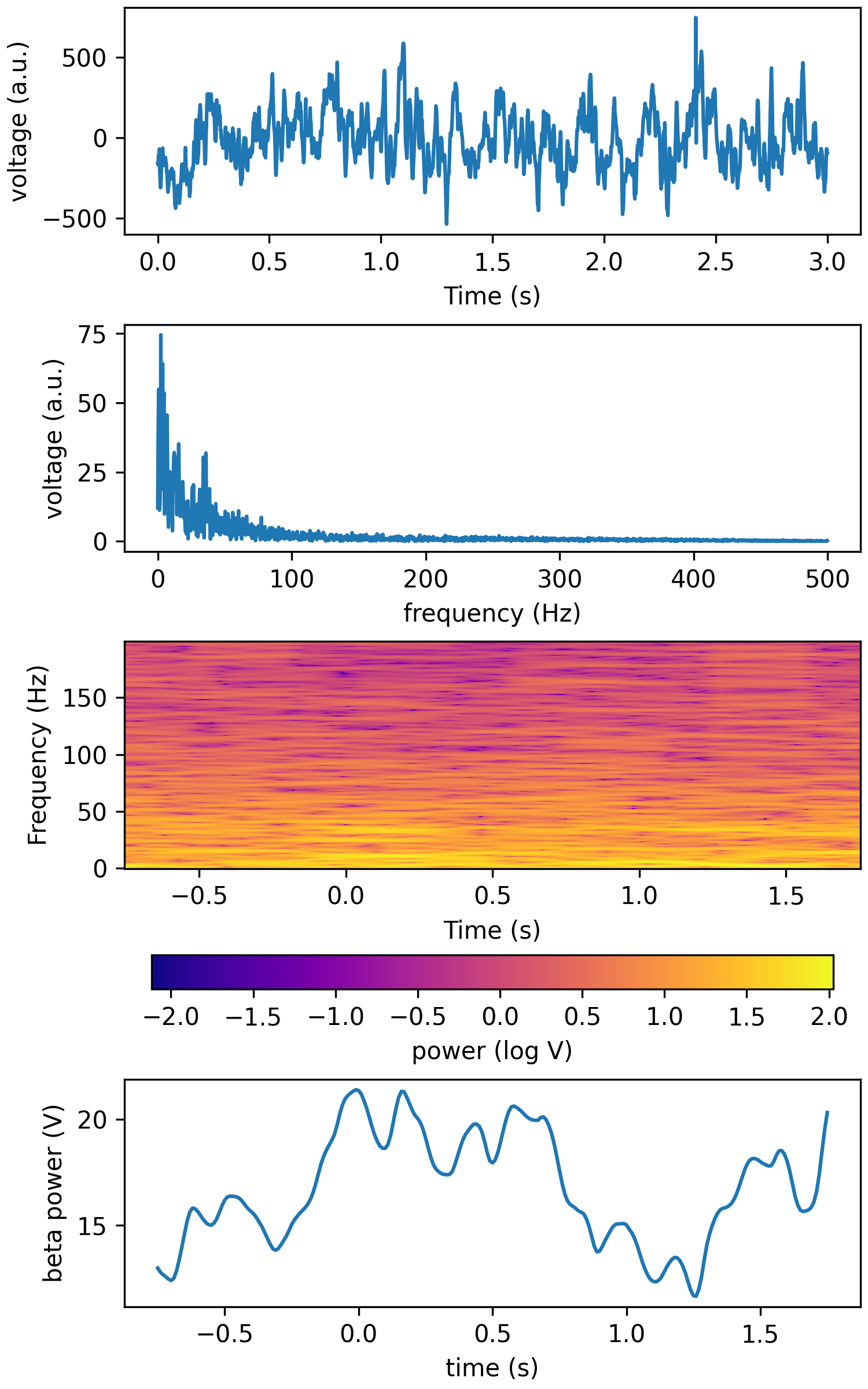
aopy.analysis.base.calc_mt_tfr(ts_data, n, p, k, fs, step=None, fk=None, pad=2, ref=True, complex_output=False, dtype='float64', nonnegative_freqs=True)

Compute multitaper time-frequency estimate from multichannel signal input. This code is adapted from the Pesaran lab tfspec.

Parameters:

• ts_data (nt, [nch, ntr]) – time series array. If nch=1, the second dimension can be omitted. If ntr=1, the third dimension can be omitted. Output spectrogram dimensions (n_freq, n_time, [nch, ntr]) will also be reduced accordingly.

• n (float) – window length in seconds

• p (float) – standardized half bandwidth in hz

• k (int) – number of DPSS tapers to use

• fs (float) – sampling rate

• step (float) – window step. Defaults to step = n/10.

• fk (float) – frequency range to return in Hz ([0, fk]). Defaults to fs/2.

• pad (int) – padding factor for the FFT. This should be 1 or a multiple of 2. For N=500, if pad=1, we pad the FFT to 512 points. If pad=2, we pad the FFT to 1024 points. If pad=4, we pad the FFT to 2024 points.

• ref (bool) – referencing flag. If True, mean of neural signals across electrodes for each time window is subtracted to remove common noise so that you can get spacially-localized signals. If you only analyze single channel data, this has to be False. This paper discuss referencing scheme https://iopscience.iop.org/article/10.1088/1741-2552/abce3c

• complex_output (bool) – if True, return the complex signal instead of magnitude. Default False.

• dtype (str) – dtype of the output. Default ‘float64’

• nonnegative_freqs (bool) – if True, only include non-negative frequencies in the output. Default True.

Returns:

Tuple containing:

f (n_freq): frequency axis for spectrogram

t (n_time): time axis for spectrogram

spec (n_freq,n_time,nch,ntr): multitaper spectrogram estimate

Return type:

tuple

Examples

from analyze/tests/analysis_tests import HelperFunctions
NW = 0.3
BW = 10
step = 0.01
fk = 50
n, p, k = aopy.precondition.convert_taper_parameters(NW, BW)
print(f"using {k} tapers length {n} half-bandwidth {p}")
tfr_fun = lambda data, fs: aopy.analysis.calc_mt_tfr(data, n, p, k, fs, step=step, fk=fk, pad=2, ref=False)
HelperFunctions.test_tfr_sines(tfr_fun)

fk = 500
tfr_fun = lambda data, fs: aopy.analysis.calc_mt_tfr(data, n, p, k, fs, step=step, fk=fk, pad=2, ref=False)
HelperFunctions.test_tfr_chirp(tfr_fun)

fk = 200
tfr_fun = lambda data, fs: aopy.analysis.calc_mt_tfr(data, n, p, k, fs, step=step, fk=fk, pad=2, ref=False, dtype='int16')
HelperFunctions.test_tfr_lfp(tfr_fun)

See also

calc_cwt_tfr()

Note

The time axis returned by calc_mt_tfr corresponds to the center of the sliding window (n seconds). To move the time axis so that the spectrogram bins are aligned to the right edge of each window, do time += n/2.

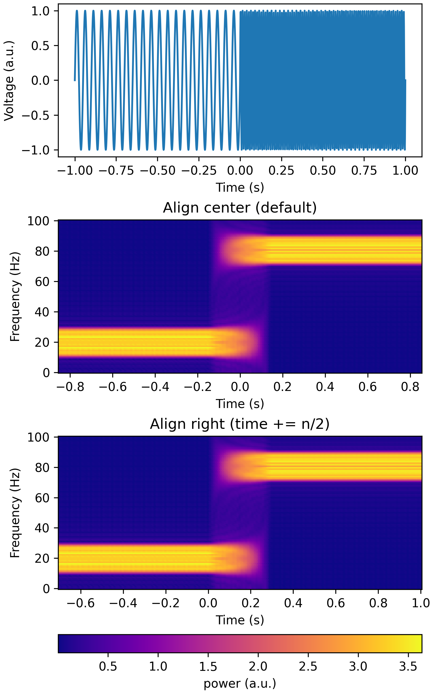
Modified September 2023 to return magnitude instead of magnitude squared power.

aopy.analysis.base.calc_rms(signal, remove_offset=True)

Root mean square of a signal

Parameters:

• signal (nt, ...) – voltage along time, other dimensions will be preserved

• remove_offset (bool) – if true, subtract the mean before calculating RMS

Returns:

rms of the signal along the first axis. output dimensions will be the same non-time dimensions as the input signal

Return type:

float array

aopy.analysis.base.calc_rolling_average(data, window_size=11, mode='copy')

Computes the rolling average of a 1- or 2-D array using a convolutional kernel. The rolling average is always applied along the first axis of the array. If mode is ‘nan’, the ends of the array where an incomplete rolling average occurs is replaced with np.nan. If mode is ‘copy’ (the default), the first and last valid datapoint (fully overlapping with the kernel) are copied backwards and forwards, respectively. The size of the output will always be the same as the size of the input data.

Parameters:

• data (nt, nch) – The array of data to compute the rolling average for.

• window_size (int) – The size of the kernel in number of samples. Must be odd.

• mode (str) – Either ‘copy’ or ‘nan’, determines what happens on the edges where the kernel doesn’t fully overlap the data

Returns:

The rolling average of the input data.

Return type:

(nt,) array

aopy.analysis.base.calc_sem(data, axis=None)

This function calculates the standard error of the mean (SEM). The SEM is calculated with the following equation where \(\sigma\) is the standard deviation and \(n\) is the number of samples. When the data matrix includes NaN values, this function ignores them when calculating the \(n\). If no value for axis is input, the SEM will be calculated across the entire input array.

\[SEM = \frac{\sigma}{\sqrt{n}}\]

Parameters:

• data (nd array) – Input data matrix of any dimension

• axis (int or tuple) – Axis to perform SEM calculation on

Returns:

SEM value(s).

Return type:

nd array

aopy.analysis.base.calc_spatial_data_correlation(elec_data, elec_pos, interp=False, grid_size=None, interp_method='cubic', align_maps=False)

Wrapper around calc_spatial_map_correlation() that interpolates electrode data onto a 2D map before computing correlation.

Parameters:

• elec_data ((nmaps,) list) – list of (nch,) spatial data arrays

• elec_pos ((nch, 2) array) – electrode positions for each channel

• interp (bool) – whether or not to interpolate data maps. Default False.

• grid_size ((2,) tuple, optional) – map size for interpolation, e.g. (16,16) for a 16x16 grid

• interp_method (str) – interpolation method to use. Default ‘cubic’

• align_maps (bool) – Whether or not to align maps. Default False.

Returns:

tuple containing:

NCC (nmaps, nmaps): normalized correlation coefficients

shifts ((nmaps,) list): list of (row_shifts, col_shifts) for each map

Return type:

tuple

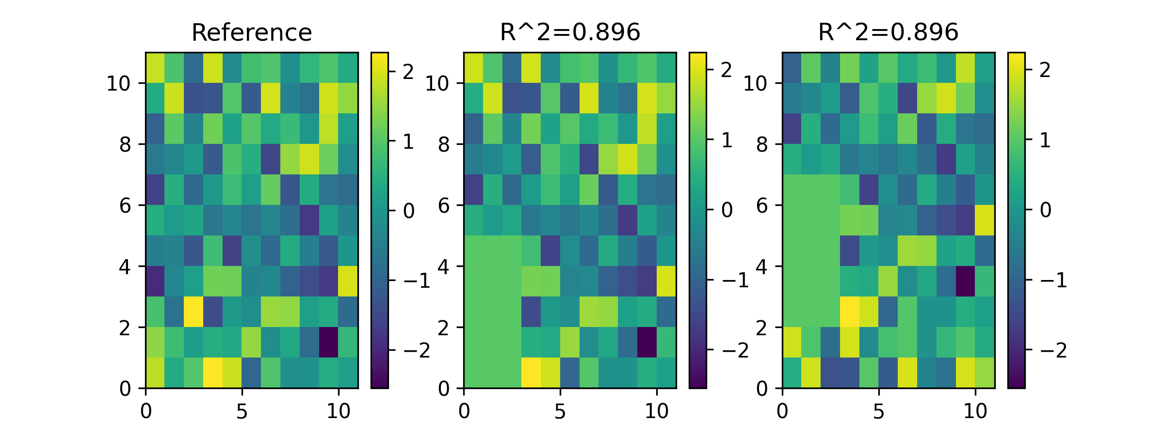
aopy.analysis.base.calc_spatial_map_correlation(data_maps, align_maps=False)

Generate a correlation matrix between all pairs of input data maps. If specified, it also aligns the input maps. Alignment is done using align_spatial_maps() which finds the location of the peak of the 2D correlation function. Here, we calculate the 1D correlation between flattened versions of the input data maps. This function removes datapoints along the second axis if any map contains NaN values at that location. Data maps are normalized by their magnitude prior to computing correlation.

Note

If shifts are unexpectedly high, there is likely not high enough correlation between the datamaps and alignment should not be used.

Parameters:

• data_maps ((nmaps,) list) – list of (ncol, nrow) spatial data arrays

• align_maps (bool) – Whether or not to align maps. Always aligns to the first map. Default False.

Returns:

tuple containing:

NCC (nmaps, nmaps): normalized correlation coefficients

shifts ((nmaps,) list): list of (row_shifts, col_shifts) for each map

Return type:

tuple

Examples

Generate a noisy map and two copies with known change and shift

data1 = np.random.normal(0,1,(nrows,ncols))
data2 = data1.copy()
NCC, _ = aopy.analysis.calc_spatial_map_correlation([data1, data2], False)
self.assertAlmostEqual(NCC[1,0], 1)

nrows_changed = 5
ncols_changed = 3
for irow in range(nrows_changed):
    data2[irow,:ncols_changed] = 1

data3 = data2.copy()
data3 = np.roll(data3, 2, axis=0)

NCC, shifts = aopy.analysis.calc_spatial_map_correlation([data1, data2, data3], True)

Plot the maps and correlation coefficients against the reference map

fig, [ax1, ax2, ax3] = plt.subplots(1,3, figsize=(8,3))
im1 = ax1.pcolor(data1)
ax1.set(title='Reference')
plt.colorbar(im1, ax=ax1)

im2 = ax2.pcolor(data2)
ax2.set(title=f'R^2={np.round(NCC[1,0],3)}')
plt.colorbar(im2, ax=ax2)

im3 = ax3.pcolor(data3)
ax3.set(title=f'R^2={np.round(NCC[2,0],3)}')
plt.colorbar(im3, ax=ax3)

aopy.analysis.base.calc_spatial_tf_data_correlation(freqs, time, tf_elec_data, elec_pos, null_tf_elec_data=None, band=(12, 150), window=(0, 1), alternative='greater', nan_policy='propagate', alpha=0.05, interp=False, grid_size=None, interp_method='cubic', align_maps=False)

Wrapper around calc_spatial_map_correlation() that averages over a given time-window and frequency-band, then interpolates data onto a 2D map before computing correlation.

Parameters:

• freqs (nfreq) – frequency axis

• time (nt) – time axis

• tf_elec_data (list of (nt, nfreq, nch)) – time-frequency data arrays

• band (tuple) – frequency band of interest, e.g. (12, 150), in Hz

• window (tuple) – time window of interest, e.g. (0, 1), in seconds

• null_tf_elec_data (list of (nt, nfreq, nch), optional) – time-frequency null data arrays to compute significance. If None, no significance testing is performed.

• alternative (str, optional) – Hypothesis test alternative (‘greater’, ‘less’, ‘two-sided’). Defaults to ‘greater’.

• nan_policy (str, optional) – Handling of NaN values. Defaults to ‘propagate’.

• alpha (float, optional) – Significance level. Defaults to 0.05.

• interp (bool) – whether or not to interpolate data maps. Default False.

• grid_size ((2,) tuple, optional) – map size for interpolation, e.g. (16,16) for a 16x16 grid

• interp_method (str) – interpolation method to use. Default ‘cubic’

• align_maps (bool) – Whether or not to align maps. Default False.

Returns:

tuple containing:

NCC (nmaps, nmaps): normalized correlation coefficients

shifts ((nmaps,) list): list of (row_shifts, col_shifts) for each map

Return type:

tuple

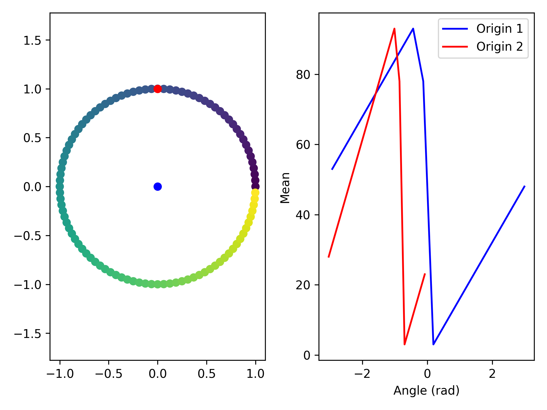
aopy.analysis.base.calc_stat_over_angle_from_pos(elec_data, elec_pos, origin, statistic='mean', bins=20)

Bins spatial data based on the angle from each electrode to the origin, then compute a statistic on the electrode data within each angular bin.

Parameters:

• elec_data (nelec) – electrode data

• elec_pos (nelec, 2) – x, y position of each electrode

• origin (2,) – x, y position to calculate angle from

• statistic (str) – statistic to calculate (‘mean’, ‘std’, ‘median’, ‘max’, ‘min’). See scipy.stats.binned_statistic. Default ‘mean’.

• bins (int or array) – number of angular bins or bin edges for binned_statistic. Default 20.

Returns:

tuple containing:

angle (nbins): angle (in radians) to origin at each bin

stat (nbins): statistic at each bin

Return type:

tuple

Example

# Create a circle of electrodes
nelec = 100
elec_data = np.arange(nelec)
elec_pos = [[np.cos(idx/nelec*2*np.pi), np.sin(idx/nelec*2*np.pi)] for idx in range(nelec)]
origin1 = [0,0]
origin2 = [0,1]

plt.figure()
plt.subplot(1,2,1)
plt.scatter(*np.array(elec_pos).T, c=elec_data)
plt.scatter(*origin1, color='b')
plt.scatter(*origin2, color='r')
plt.axis('equal')

angle, mean = aopy.analysis.calc_stat_over_angle_from_pos(elec_data, elec_pos, origin1)
plt.subplot(1,2,2)
plt.plot(angle, mean, color='b')
angle, mean = aopy.analysis.calc_stat_over_angle_from_pos(elec_data, elec_pos, origin2)
plt.plot(angle, mean, color='r')
plt.xlabel('Angle (rad)')
plt.ylabel('Mean')

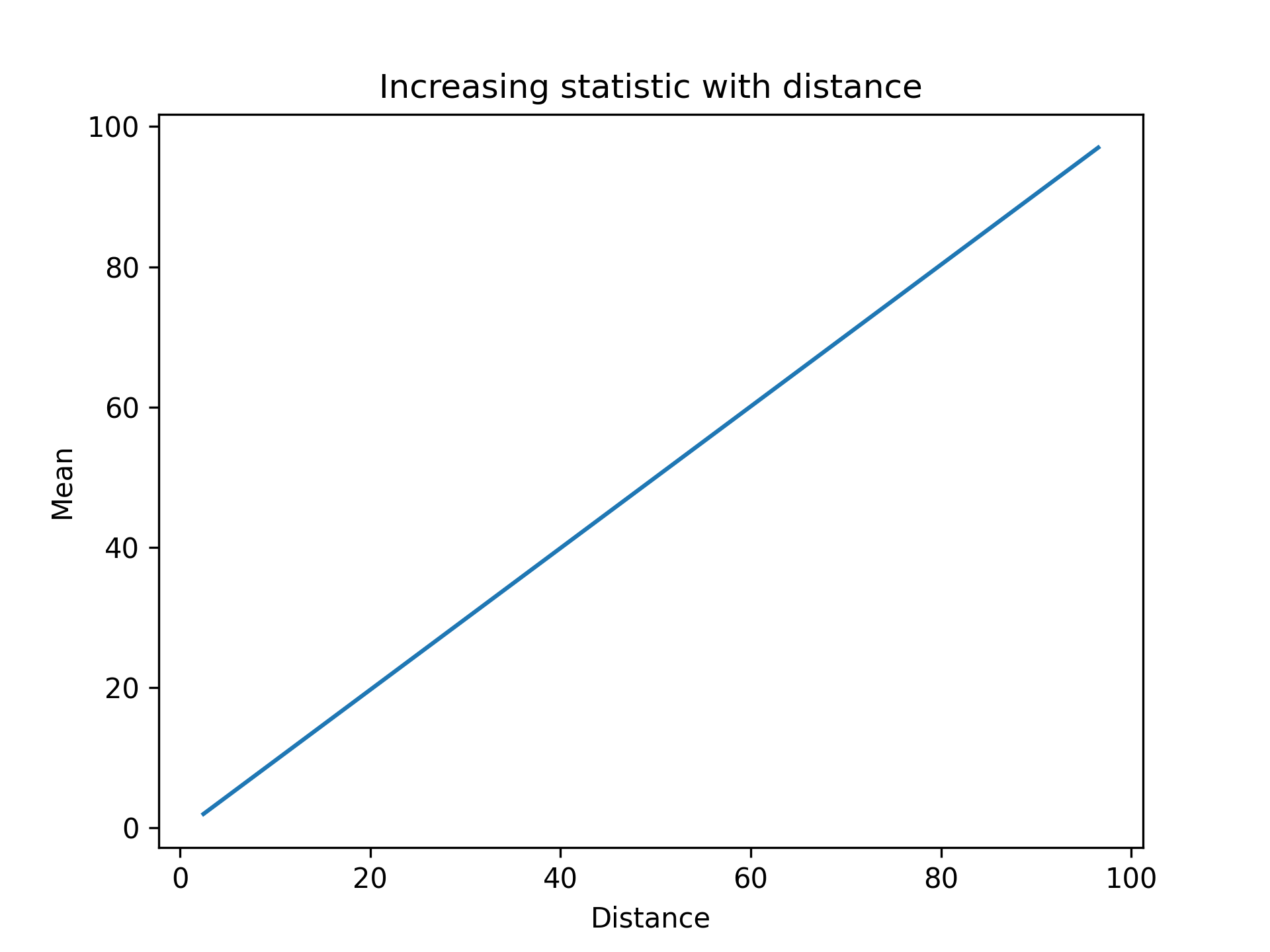
aopy.analysis.base.calc_stat_over_dist_from_pos(elec_data, elec_pos, pos, statistic='mean', bins=20)

For spatial data, calculate a statistic over distance from a given position.

Parameters:

• elec_data (nelec) – electrode data

• elec_pos (nelec, 2) – x, y position of each electrode

• pos (2,) – x, y position to calculate distance from

• statistic (str) – statistic to calculate (‘mean’, ‘std’, ‘median’, ‘max’, ‘min’). See scipy.stats.binned_statistic. Default ‘mean’.

• bins (int or array) – number of bins or bin edges for binned_statistic. Default 20.

Returns:

tuple containing:

dist (nbins): electrode distance at each bin

stat (nbins): statistic at each bin

Return type:

tuple

Example

nelec = 100
elec_data = np.arange(nelec)
elec_pos = [[idx, 1] for idx in range(nelec)]
pos = [0,1]
dist, mean = aopy.analysis.calc_stat_over_dist_from_pos(elec_data, elec_pos, pos)

plt.figure()
plt.plot(dist, mean)
plt.xlabel('Distance')
plt.ylabel('Mean')
plt.title('Increasing statistic with distance')

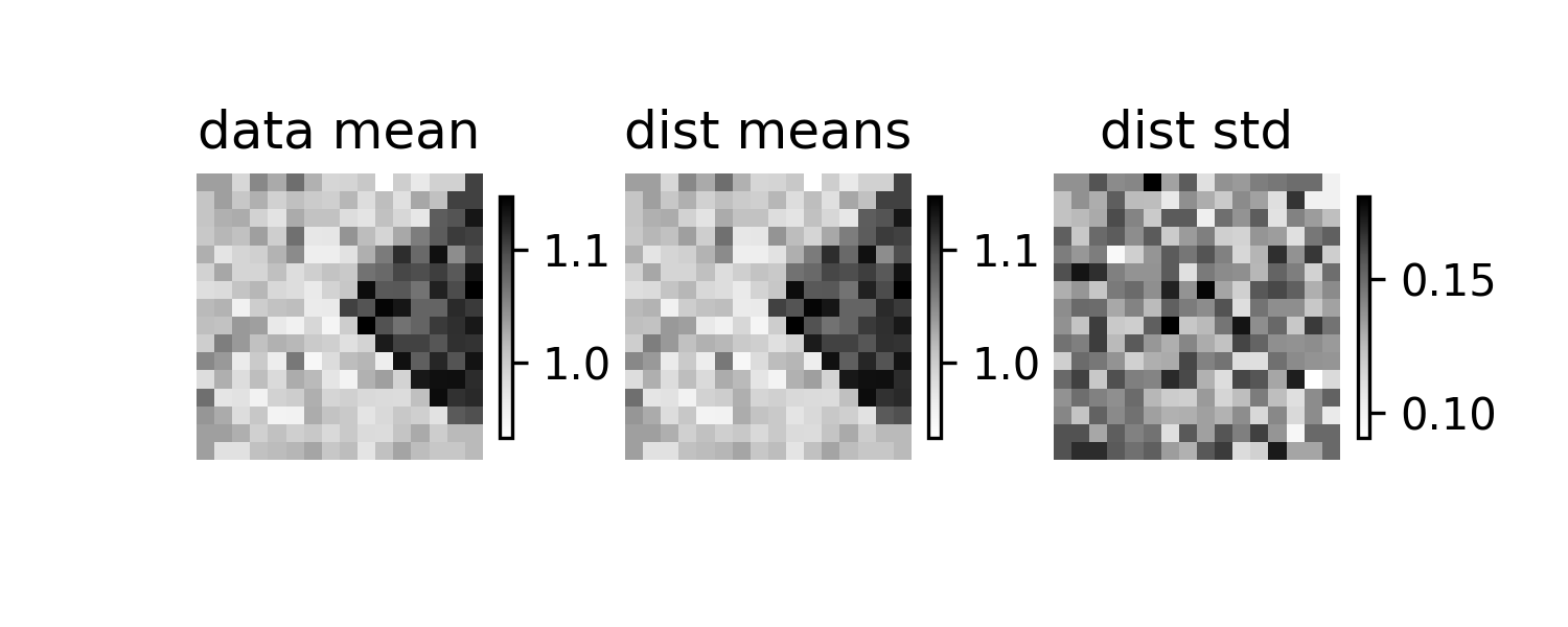
aopy.analysis.base.calc_statistic_random_trials(data, n_trials=300, statistic=functools.partial(numpy.mean, axis=0), rng=None)

Calculate a distribution of a statistic across groups of trials of the data by randomly sampling trials without replacement.

Parameters:

• data (ntrials, nch) – data to calculate the statistic on. Also accepts a pandas DataFrame of shape (ntrials, …) if the statistic can be calculated on a DataFrame.

• n_trials (int) – number of trials to use in each bootstrap

• statistic (function) – function to calculate the statistic on the data. Should take the form f(x) = y where x is a 2D array of shape (n_trials, nch) and y is a 1D array of shape (nch). Default is np.mean(x, axis=0).

• rng (numpy.random.Generator, optional) – Random number generator to use for shuffling trials. If None, uses the default random number generator. Default is None.

Returns:

distributions of the statistic across divisions of the data.

Return type:

(len(data)//ntrials, nch) array

Examples

elec_pos, _, _ = aopy.data.load_chmap()
n_elec = len(elec_pos)
total_trials = 1600
n_trials = 50
np.random.seed()
data = 0.5*np.ones((total_trials,n_elec))
data += np.random.normal(0.5, size=(total_trials,n_elec))
data[:,n_elec//4:n_elec//2] += 0.1

dists = aopy.analysis.calc_statistic_random_trials(data, n_trials=n_trials)
self.assertEqual(np.shape(dists), (len(data)//n_trials, n_elec))

# Test that the distribution means are close to the original data mean
mean = np.mean(data, axis=0)
dists_mean = np.mean(dists, axis=0)
dists_std = np.std(dists, axis=0)
for i in range(n_elec):
    self.assertAlmostEqual(mean[i], dists_mean[i], delta=0.1)
clim = (np.min(dists_mean), np.max(dists_mean))

plt.figure(figsize=(5,2), dpi=300)
plt.subplot(1,3,1)
im = aopy.visualization.plot_spatial_drive_map(mean,
                                elec_data=True, cmap='Grays')
im.set_clim(*clim)
plt.axis('off')
plt.colorbar(im, shrink=0.5)
plt.title('data mean')

plt.subplot(1,3,2)
im = aopy.visualization.plot_spatial_drive_map(dists_mean,
                                elec_data=True, cmap='Grays')
im.set_clim(*clim)
plt.axis('off')
plt.colorbar(im, shrink=0.5)
plt.title('dist means')

plt.subplot(1,3,3)
im = aopy.visualization.plot_spatial_drive_map(dists_std,
                                elec_data=True, cmap='Grays')
plt.axis('off')
plt.colorbar(im, shrink=0.5)
plt.title('dist std')

aopy.analysis.base.calc_task_rel_dims(neural_data, kin_data, conc_proj_data=False)

Calculates the task relevant dimensions by regressing neural activity against kinematic data using least squares. If the input neural data is 3D, all trials will be concatenated to calculate the subspace. Calculation is based on the approach used in Sun et al. 2022 https://doi.org/10.1038/s41586-021-04329-x

\[R \in \mathbb{R}^{nt \times nch}\]

\[M \in \mathbb{R}^{nt \times ndim}\]

\[\beta \in \mathbb{R}^{nch \times ndim}\]

\[R = M\beta^T\]

\[[\beta_0 \beta_x \beta_y]^T = (M^T M)^{-1} M^T R\]

Parameters:

• neural_data ((nt, nch) or list of (nt, nch)) – Input neural data (\(R\)) to regress against kinematic activity.

• kin_data ((nt, ndim) or list of (nt, ndim)) – Kinematic variables (\(M\)), commonly position or instantaneous velocity. ‘ndims’ refers to the number of physical dimensions that define the kinematic data (i.e. X and Y)

• conc_proj_data (bool) – If the projected neural data should be concatenated.

Returns:

Tuple containing:

(nch, ndim): Subspace (\(\beta\)) that best predicts kinematic variables. Note the first column represents the intercept, then the next dimensions represent the behvaioral variables

((nt, nch) or list of (nt, ndim)): Neural data projected onto task relevant subspace

Return type:

tuple

aopy.analysis.base.calc_tfr_mean(freqs, time, spec, band=(0, 1e+16), window=(-1e+16, 1e+16))

Calculate the mean within a specific frequency band and time window.

Parameters:

• freqs (nfreq,) – Frequency values in Hz.

• time (nt,) – Time values in seconds.

• spec (nfreq, nt, nch) – Time-frequency spectrogram data.

• band (tuple) – Frequency band (low, high) in Hz. Defaults to (0, np.inf).

• window (tuple, optional) – Time window (start, end) in seconds. Defaults to (-np.inf, np.inf).

Returns:

Mean spectral value within the specified band and time window for each channel.

Return type:

(nch,)

aopy.analysis.base.calc_tfr_mean_fdrc_ranktest(freqs, time, spec, null_specs, band=(0, 1e+16), window=(-1e+16, 1e+16), alternative='greater', nan_policy='raise', alpha=0.05)

Compute band-specific Wilcoxon sign-rank test with false discovery-rate correction. Used for comparing coherence maps against null distributions. Spectrograms must be multi-channel.

Parameters:

• freqs (nfreq,) – Frequency axis in Hz.

• time (nt,) – Time axis in seconds.

• spec (nfreq, nt, nch) – Observed spectrogram.

• null_specs (n_null, nfreq, nt, nch) – Distribution of null spectrograms.

• band (tuple, optional) – Frequency band (low, high) in Hz. Defaults to (0, np.inf).

• window (tuple, optional) – Time window (start, end) in seconds. Defaults to (-np.inf, np.inf).

• alternative (str, optional) – Hypothesis test alternative. See scipy.stats.calc_fdrc_ranktest for options. Defaults to ‘greater’.

• nan_policy (str, optional) – Handling of NaN values. See scipy.stats.calc_fdrc_ranktest for options. Defaults to ‘raise’.

• alpha (float, optional) – Significance level. Defaults to 0.05.

Returns:

tuple containing:

• diff (nch,): Effect size at each channel.

• p_fdrc (nch,): Adjusted p-values at each channel.

Return type:

tuple

aopy.analysis.base.calc_trial_bootstraps(data, n_trials=300, n_bootstraps=30, statistic=functools.partial(numpy.mean, axis=0), rng=None, parallel=False, verbose=True)

Repeatedly call calc_statistic_random_trials() to generate statistics over randomly sampled trials. Each bootstrap draws random groups of trials, each of size n_trials, without replacement, until there aren’t enough trials to make another full size group. The statistic is then calculated on each group, resulting in n_bootstraps * len(data)//n_trials values.

Parameters:

• data (ntrials, nch) – data to calculate the statistic on

• n_trials (int) – number of trials to use in each bootstrap

• n_bootstraps (int) – number of bootstrap trials to perform

• statistic (function) – function to calculate the statistic on the data. Should take the form f(x) = y where x is a 2D array of shape (n_trials, nch) and y is a 1D array of shape (nch). Default is np.mean(x, axis=0).

• rng (numpy.random.Generator, optional) – Random number generator to use for shuffling trials. Be careful when using this with parallel processing, as it may lead to duplicate results if the same random number generator is used across processes. If None, uses a new default random number generator on each bootstrap. Default is None.

• parallel (bool or mp.pool.Pool, optional) – Whether to run the bootstraps in parallel. If True, uses a multiprocessing pool with 10 workers. If a Pool is provided, it will use that pool instead. The pool will not be closed. If False, runs the bootstraps sequentially.

• verbose (bool, optional) – Whether to print progress bars. Default is True.

Returns:

multiple bootstraps of distributions

of the statistic applied to divisions of the data.

Return type:

(n_bootstraps, len(data)//n_trials, nch) array

aopy.analysis.base.calc_tsa_mt_tfr(data, fs, win_t, step_t, bw=None, f_max=None, pad=2, jackknife=False, adaptive=False, sides='onesided')

Compute multitaper time-frequency power estimate from multichannel signal input. This code uses nitime time-series analysis below. In comparison to calc_mt_tfr() this function is very slow.

Parameters:

• data (nt, nch) – nd array of input neural data (multichannel)

• fs (int) – sampling rate

• win_t (float) – spectrogram window length (in seconds)

• step_t (float) – step size between spectrogram windows (in seconds)

• bw (float, optional) – spectrogram frequency bin bandwidth. Defaults to None.

• f_max (float) – frequency range to return in Hz ([0, f_max]). Defaults to samplerate/2.

• pad (int) – padding factor for the FFT. This should be 1 or a multiple of 2. For N=500, if pad=1, we pad the FFT to 512 points. If pad=2, we pad the FFT to 1024 points. If pad=4, we pad the FFT to 2024 points.

• adaptive (bool, optional) – adaptive taper weighting. Defaults to False.

Returns:

Tuple containing:

freqs (nfreq,): spectrogram frequency array (equal in length to win_t * fs // 2 + 1)

time (nt,): spectrogram time array (equal in length to (len(data)/fs - win_t)/step_t)

**spec (nfreq, nt, nch): multitaper spectrogram estimate. Last dimension squeezed for 1-d inputs.

Return type:

tuple

Examples

from analyze/tests/analysis_tests import HelperFunctions
win_t = 0.3
step_t = 0.01
bw = 20
fk = 50
tfr_fun = lambda data, fs: aopy.analysis.calc_tsa_mt_tfr(data, fs, win_t, step_t, bw=bw, f_max=fk)
HelperFunctions.test_tfr_sines(tfr_fun)

fk = 500
tfr_fun = lambda data, fs: aopy.analysis.calc_tsa_mt_tfr(data, fs, win_t, step_t, bw=bw, f_max=fk)
HelperFunctions.test_tfr_chirp(tfr_fun)

fk = 200
tfr_fun = lambda data, fs: aopy.analysis.calc_tsa_mt_tfr(data, fs, win_t, step_t, bw=bw, f_max=fk)
HelperFunctions.test_tfr_lfp(tfr_fun)

aopy.analysis.base.calc_welch_psd(data, fs, n_freq=None)

Computes power using Welch’s method. Welch’s method computes an estimate of the power by dividing the data into overlapping segments, computes a modified periodogram for each segment and then averages the periodogram. Periodogram is averaged using median.

Parameters:

• data (nt, ...) – time series data.

• fs (float) – sampling rate

• n_freq (int) – no. of frequency points expected

Returns:

Tuple containing:

f (nfft): frequency points vector

psd_est (nfft, …): estimated power spectral density (PSD)

Return type:

tuple

aopy.analysis.base.classify_by_lda(X_train_lda, y_class_train, n_splits=5, n_repeats=3, random_state=1)

Trains a linear discriminant model on the training data (X_train_lda) and their labels (y_class_train) with data spliting and k-fold validation. Returns accuracy and variance based on how well the model is able to predict the left-out data.

Parameters:

• X_train_lda (n_classes, n_features) – 2d training data. first dimension is the number of examples, second dimension is the size of each example

• y_class_train (n_classes) – class to which each example belongs

• n_splits (int, optional) – number of paritions to split data Defaults to 5.

• n_repeats (int, optional) – number of repeated fitting Defaults to 3.

• random_state (int, optional) – random state for data spliting Defaults to 1.

Returns:

Tuple containing:

accuracy (float): mean accuracy of the repeated lda runs. std (float): standard deviation of the repeated lda runs.

Return type:

tuple

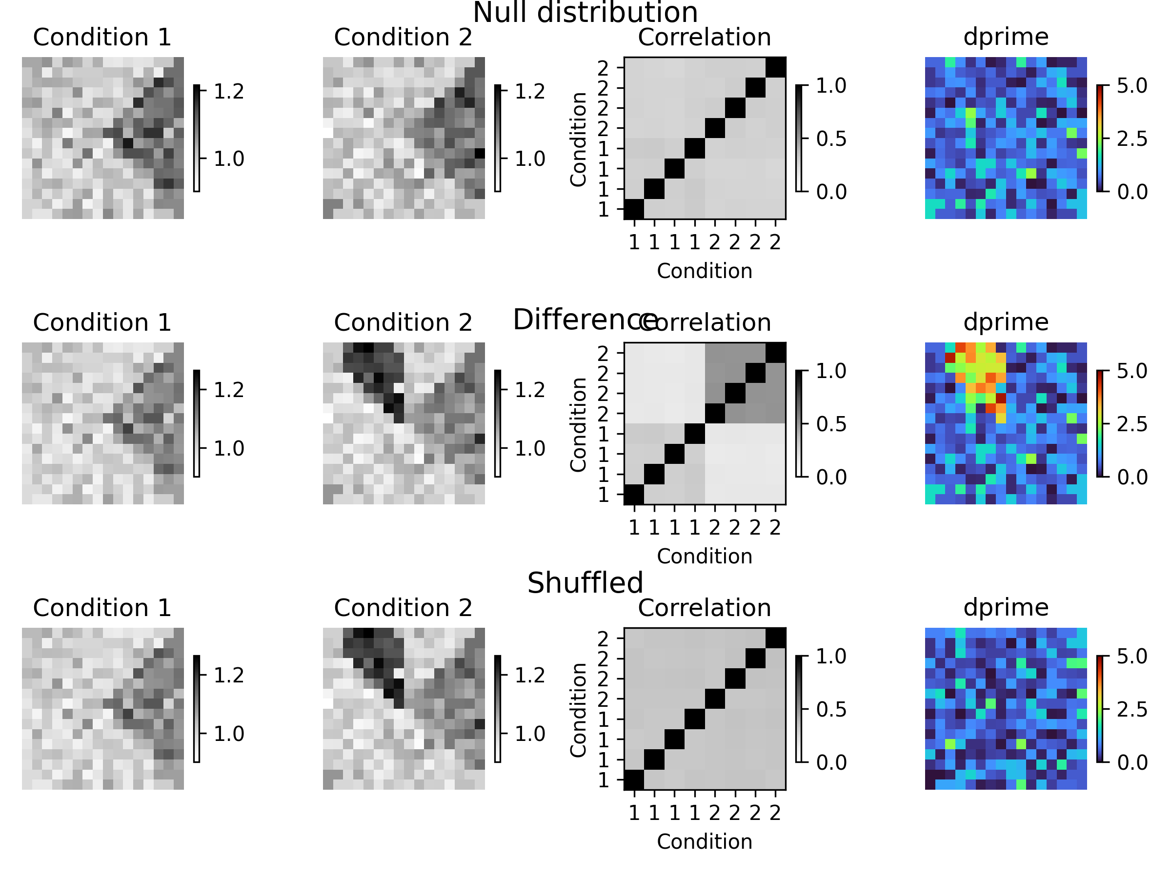
aopy.analysis.base.compare_conditions_bootstrap_spatial_corr(data, elec_pos, labels, n_trials=300, n_bootstraps=30, n_shuffle=0, statistics=functools.partial(numpy.mean, axis=0), rng=None, parallel=False)

Compare multiple conditions using bootstrapping and shuffling. Each additional bootstrap draws random groups of trials, each of size n_trials, without replacement, until there aren’t enough trials to make another full size group. The statistic is then calculated on each group, resulting in n_bootstraps * len(data)//n_trials values. The spatial correlation of the statistic across conditions is calculated within each bootstrap, and the d-prime is calculated for all statistics pooled across bootstraps. Finally, if n_shuffle > 0, the labels are shuffled n_shuffle times and the bootstrap procedure repeated to create a null distribution for the spatial correlation and d-prime values.

Parameters:

• data (ntrials, nch) – data to calculate the statistic on

• elec_pos ((nch, 2) array) – electrode positions for each channel

• labels (ntrials,) – labels for each trial, used to group trials by condition

• n_trials (int) – number of trials to use in each bootstrap

• n_bootstraps (int) – number of bootstrap trials to perform

• n_shuffle (int) – number of times to shuffle the labels to create a null distribution

• statistics (function or list of functions) – function(s) to calculate the statistic on the data. If more than one is supplied, they will be applied per condition

• rng (numpy.random.Generator, optional) – Random number generator to use for shuffling trials. Be careful when using this with parallel processing, as it may lead to duplicate results if the same random number generator is used across processes. If None, uses a new default random number generator on each bootstrap. Default is None.

• parallel (bool or mp.pool.Pool, optional) – Whether to run the bootstraps in parallel. If True, uses a multiprocessing pool with 10 workers. If a Pool is provided, it will use that pool instead. The pool will not be closed. If False, runs the bootstraps sequentially. Default is False.

Returns:

tuple containing:

observed_dists (n_cond, n_bootstraps, len(data)//n_trials, nch): bootstraps distributions for each condition

conditions (n_cond): unique conditions in the labels

observed_corr (n_bootstraps, n_cond*n_cond, n_cond*n_cond, nch): list of spatial correlation matrices for each bootstrap

observed_dprime (nch): d-prime value for each channel pooled across bootstraps and comparing across conditions

if n_shuffle > 0:

shuff_dists_dist (n_shuffle, n_cond, n_bootstraps, len(data)//n_trials, nch): shuffled distributions for each condition

shuff_corr_dist (n_shuffle, n_bootstraps, n_cond*n_cond, n_cond*n_cond, nch): shuffled spatial correlation matrices

shuff_dprime_dist (n_shuffle, nch): shuffled d-prime

Return type:

tuple

Examples

elec_pos, _, _ = aopy.data.load_chmap()
n_elec = len(elec_pos)
total_trials = 1600
n_trials = 200
n_bootstraps = 50

# Test null distribution
np.random.seed(0)
data = 0.5*np.ones((total_trials,n_elec))
data += np.random.normal(0.5, size=(total_trials,n_elec))
data[:,n_elec//4:n_elec//2] += 0.1
labels = np.zeros((total_trials,))
labels[total_trials//2:] = 1

def plot_result(means, corr_mat, dprime, row):

    mean12 = np.concatenate(means)
    clim = (np.min(mean12),np.max(mean12))

    plt.subplot(3,4,(4*(row-1))+1)
    im = aopy.visualization.plot_spatial_drive_map(means[0],
                                    elec_data=True, cmap='Grays')
    im.set_clim(*clim)
    plt.colorbar(im, shrink=0.5)
    plt.axis('off')
    plt.title('Condition 1')

    plt.subplot(3,4,(4*(row-1))+2)
    im = aopy.visualization.plot_spatial_drive_map(means[1],
                                    elec_data=True, cmap='Grays')
    im.set_clim(*clim)
    plt.colorbar(im, shrink=0.5)
    plt.axis('off')
    plt.title('Condition 2')

    plt.subplot(3,4,(4*(row-1))+3)
    im = plt.imshow(np.nanmean(corr_mat, axis=0), cmap='Grays', vmin=0, vmax=1, origin='lower')
    plt.colorbar(im, shrink=0.5)
    sz = len(corr_mat[0])//2
    plt.xticks(range(sz*2), labels=['1']*sz + ['2']*sz)
    plt.yticks(range(sz*2), labels=['1']*sz + ['2']*sz)
    plt.xlabel('Condition')
    plt.ylabel('Condition')
    plt.title('Correlation')

    plt.subplot(3,4,(4*(row-1))+4)
    im = aopy.visualization.plot_spatial_drive_map(dprime, elec_data=True, cmap='turbo')
    im.set_clim(0,5)
    plt.axis('off')
    plt.colorbar(im, shrink=0.5)
    plt.title('dprime')

fig = plt.figure(figsize=(8,6), dpi=300)

means = [np.mean(data[labels == i,:], axis=0) for i in np.unique(labels)]
dists, conditions, corr_mat, dprime =                 aopy.analysis.compare_conditions_bootstrap_spatial_corr(
        data, elec_pos, labels, n_trials=n_trials, n_bootstraps=n_bootstraps, parallel=False
    )
plot_result(means, corr_mat, dprime, 1)
fig.text(0.5, 1, "Null distribution", ha='center', va='top', fontsize=14)

# Test difference
data[labels == 1,:n_elec//8] += 0.2

means = [np.mean(data[labels == i,:], axis=0) for i in np.unique(labels)]
dists, conditions, corr_mat, dprime, shuff_dists, shuff_mat, shuff_dprime =                 aopy.analysis.compare_conditions_bootstrap_spatial_corr(
        data, elec_pos, labels, n_trials=n_trials, n_bootstraps=n_bootstraps, n_shuffle=1, parallel=False
    )
plot_result(means, corr_mat, dprime, 2)
fig.text(0.5, 0.65, "Difference", ha='center', va='top', fontsize=14)

# Test shuffled
plot_result(means, shuff_mat[0], shuff_dprime[0], 3)
fig.text(0.5, 0.35, "Shuffled", ha='center', va='top', fontsize=14)

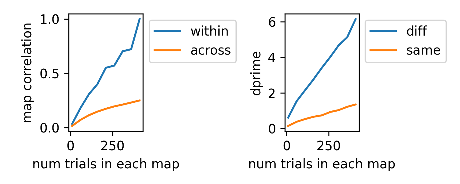
Sweep over increasing n_trials of the same data as above

n_bootstraps = 10
avg_coeff_1 = []
avg_coeff_2 = []
avg_dprime_1 = []
avg_dprime_2 = []
trial_sizes = range(10, 450, 50)
for n_trials in trial_sizes:
    dists, conditions, corr_mat, dprime =                     aopy.analysis.compare_conditions_bootstrap_spatial_corr(
            data, elec_pos, labels, n_trials=n_trials, n_bootstraps=n_bootstraps, parallel=False
        )
    avg_corr_map = np.nanmean(corr_mat, axis=0)
    sz = avg_corr_map.shape[0]//2
    avg_coeff_1.append(np.nanmean(avg_corr_map[:sz,:sz]))
    avg_coeff_2.append(np.nanmean(avg_corr_map[sz:,:sz]))
    avg_dprime_1.append(np.mean(dprime[:n_elec//8]))
    avg_dprime_2.append(np.mean(dprime[-n_elec//8:]))

plt.figure(figsize=(5,2), dpi=300)
plt.subplot(1,2,1)
plt.plot(trial_sizes, avg_coeff_1)
plt.plot(trial_sizes, avg_coeff_2)
plt.ylabel('map correlation')
plt.xlabel('num trials in each map')
plt.legend(['within', 'across'], bbox_to_anchor=[1,1], loc='upper left')

plt.subplot(1,2,2)
plt.plot(trial_sizes, avg_dprime_1)
plt.plot(trial_sizes, avg_dprime_2)
plt.ylabel('dprime')
plt.xlabel('num trials in each map')
plt.legend(['diff', 'same'], bbox_to_anchor=[1,1], loc='upper left')

plt.tight_layout()

aopy.analysis.base.factor_analysis_dimensionality_score(data_in, dimensions, nfold, maxiter=1000, verbose=False)

Estimate the latent dimensionality of an input dataset by appling cross validated factor analysis (FA) to input data and returning the maximum likelihood values.

Parameters:

• data_in (nt, nch) – Time series data in

• dimensions (ndim) – 1D Array of dimensions to compute FA for

• nfold (int) – Number of cross validation folds to compute. Must be >= 1

• maxiter (int) – Maximum number of FA iterations to compute if there is no convergence. Defaults to 1000.

• verbose (bool) – Display % of dimensions completed. Defaults to False

Returns:

Tuple containing:

log_likelihood_score (ndim, nfold): Array of MLE FA score for each dimension for each fold

iterations_required (ndim, nfold): How many iterations of FA were required to converge for each fold

Return type:

tuple

aopy.analysis.base.find_outliers(data, std_threshold)

Use kmeans clustering to find the center point of a dataset and distances from each data point to the center point. Data points further than a specified number of standard deviations away from the center point are labeled as outliers. This is particularily useful for high dimensional data

Note: This function only uses the kmeans function to calculate centerpoint distances but does not output any useful information about data clusters.

Example:

>>> data = np.array([[0.5,0.5], [0.75,0.75], [1,1], [10,10]])
>>> outliers_labels, distance = aopy.analysis.find_outliers(data, 2)
>>> print(outliers_labels, distance)
[True, True, True, False] [3.6239, 3.2703, 2.9168, 9.8111]

Parameters:

• data (n, nfeatures) – Input data to plot in an nfeature dimensional space and compute outliers

• std_threshold (float) – Number of standard deviations away a data point is required to be to be classified as an outlier

Returns:

Tuple containing:

good_data_idx (n): Labels each data point if it is an outlier (True = good, False = outlier)

distances (n): Distance of each data point from center

Return type:

tuple

aopy.analysis.base.fit_linear_regression(X: numpy.ndarray, Y: numpy.ndarray, coefficient_coeff_warning_level: float = 0.5) → numpy.ndarray

Function that fits a linear regression to each matching column of X and Y arrays.

Parameters:

• [np.ndarray] (Y) – number of data points by number of columns. columns of independant vars.

• [np.ndarray] – number of data points by number of columns. columns of dependant vars

• coeffcient_coeff_warning_level (float) – if any column returns a corr coeff less than this level

Returns:

tuple containing:

slope (n_columns): slope of each fit

intercept (n_columns): intercept of each fit

corr_coefficient (n_columns): corr_coefficient of each fit

Return type:

tuple

aopy.analysis.base.get_bandpower_feats(data, samplerate, bands, method='mt', log=False, epsilon=0, **kwargs)

Wrapper around get_tfr_feats and calc_mt_tfr.

Parameters:

• data (nt, ...) – time series data.

• samplerate (float) – sampling rate of the data.

• bands (list of tuples) – frequency bands of interest in Hz, e.g. [(0, 10), (10, 20), (130, 140)]

• log (bool) – boolean to select whether band power should be in log scale or not

• epsilon (float) – small number, e.g. 1e-10 to add to power before averaging in case there are zero values

• kwargs (dict, optional) – keyword arguments for the calc_tfr function of choice (see Note).

Raises:

ValueError – if the requested method is not valid

Returns:

tuple containing:

time (nstep): the resulting time axis for the features

feats (nfeatures, nstep, nch): band power features

Return type:

tuple

Note

For method ‘mt’, you must pass the following keyword arguments:

n (float): window length in seconds

p (float): standardized half bandwidth in hz

k (int): number of DPSS tapers to use

step (float): window step. Defaults to step = n/10.

fk (float): frequency range to return in Hz ([0, fk]). Defaults to fs/2.

Optionally you may also pass:

pad (int): padding factor for the FFT. This should be 1 or a multiple of 2.

ref (bool): referencing flag. If True, mean of neural signals across electrodes

dtype (str): dtype of the output. Default ‘float64’

aopy.analysis.base.get_confidence_interval(sample, hist_bins, alpha=0.025, ax=None, **kwarg)

Compute a confidence interval from samples, not the mean of samples If you want to compute it for the mean of samples, use scipy.stats.t.interval.

Parameters:

• sample (nsamples) – data samples

• hist_bins (int or sequence of scalars) – the number of bins or array of bin edges

• alpha (float) – significance level to define a confidece interval. Defaults to 0.025

• ax (pyplot.Axes, optional) – axis on which to plot data histogram and confidence interval. Defaults to None.

• kwargs (dict) – additional keyword arguments to pass to ax.hist()

Returns:

lower and upper bounds in the confidence interval

Return type:

(list)

aopy.analysis.base.get_empirical_pvalue(data_distribution, data_sample, test_type='two_sided', assume_gaussian=False, nbins=None)

Calculates the cumulative density function (CDF) from the input data distribution, then calculates the probability (p-value) that a data sample is part of that distribution.

Parameters:

• data_distribution (npts) – Distribution of empirically determined data points

• data_sample (npts) – Data sample(s) to get pvalue of

• test_type (str) – ‘two_sided’, ‘lower’, or ‘upper’.

• assume_gaussian (bool) – Assumes the data represents a gaussian distribution when calculating the pvalue

• nbins (int) – Number of bins to use to calculate the data distribution. Default is len(data_distribution)/100 if input is None (if necessary)

Returns:

pvalue of the input data_sample based the parameters of the input data_distribution

Return type:

significance (float)

aopy.analysis.base.get_max_erp(erp, time_before, time_after, samplerate, max_search_window=None, trial_average=False)

Finds the maximum (across time) mean (across trials) values for the given trial-aligned data or event-related potential (ERP). Identical to calc_max_erp() except this function takes trial-aligned data as input instead of timeseries data.

Parameters:

• erp ((nt, nch, ntr) array) – trial-aligned data

• time_before (float) – number of seconds to include before each event

• time_after (float) – number of seconds to include after each event

• samplerate (float) – sampling rate of the data

• max_search_window ((2,) float, optional) – range of time to search for maximum value (in seconds after event). Default is the entire time_after period.

• trial_average (bool, optional) – if True, average across trials before calculating max (using nanmean). Default False.

Returns:

array of maximum mean-ERP for each channel during the given time periods

Return type:

(nch, ntr)

aopy.analysis.base.get_pca_dimensions(data, max_dims=None, VAF=0.9, project_data=False)

Use PCA to estimate the dimensionality required to account for the variance in the given data. If requested it also projects the data onto those dimensions.

Parameters:

• data (nt, nch) – time series data where each channel is considered a ‘feature’ (nt=n_samples, nch=n_features)

• max_dims (int) – (default None) the maximum number of dimensions to reduce data onto.

• VAF (float) – (default 0.9) variance accounted for (VAF)

• project_data (bool) – (default False). If the function should project the high dimensional input data onto the calculated number of dimensions

Returns:

Tuple containing:

explained_variance (list ndims long): variance accounted for by each principal component

num_dims (int): number of principal components required to account for variance

projected_data (nt, ndims): Data projected onto the dimensions required to explain the input variance fraction. If the input ‘project_data=False’, the function will return ‘projected_data=None’

Return type:

tuple

aopy.analysis.base.get_random_timestamps(nshuffled_points, max_time, min_time=0, time_samplerate=None)

This calculates random timestamps either within a range or from a discrete time axis.

Parameters:

• nshuffled_points (int) – How many randomly selected time points to

• max_time (float) – Max of time range to draw samples from (inclusive)

• min_time (float) – Min of time range to draw samples from. Defaults to 0

• time_samplerate (int) – Samplerate [samples/s] for the time range. Defaults to None. If None, a random time to machine precision will be calculated. If a value is input, the random samples will be in increments of the samplerate (without replacement).

Returns:

Ordered random timestamps

Return type:

shuffled_timestamps (nshuffled_points)

aopy.analysis.base.get_tfr_feats(freqs, spec, bands, log=False, epsilon=1e-09)

Estimate band power in specified frequency bands, preserving other dimensions.

Parameters:

• f (nfreq,) – Frequency points vector

• spec (nfreq, nt, nch) – spectrogram of data

• bands (list of tuples) – frequency bands of interest in Hz, e.g. [(0, 10), (10, 20), (130, 140)]

• log (bool, optional) – boolean to select whether band power should be in log scale or not

• epsilon (float, optional) – small number to avoid division by zero. Default 1e-9.

Returns:

band power features at each timepoint for each channel

Return type:

lfp_power (n_features, nt, nch)

aopy.analysis.base.interp_nans(x)

Interpolate NaN values from multichannel data using linear interpolation.

Parameters:

x (n_sample, n_ch) – input data array containing nan-valued missing entries

Returns:

interpolated data, uses numpy.interp method.

Return type:

x_interp (n_sample, n_ch)

aopy.analysis.base.interpolate_extremum_poly2(extremum_idx, data, extrap_peaks=False)

This function finds the extremum approximation around an index by fitting a second order polynomial (using a lagrange polynomial) to the index input, the point before, and the point after it. In the case where the input index is either at the end or the beginning of the data array, the function can either fit the data using the closest 3 data points and return the extrapolated peak value or just return the input index. This extrapolation functionality is controlled with the ‘extrap_peaks’ input variable. Note: the extrapolation function may choose an index within the input data length if chosen points result in a polynomial with an extremum at that point.

Parameters:

• extremum_idx (int) – Current extremum index

• data (n) – data used to interpolate (or extrapolate) with

• extrap_peaks (bool) – If the extremum_idx is at the start or end of the data, indicate if the closest 3 points should be used to extrapolate a peak index.

Returns:

A tuple containing

extremum_time (float): Interpolated (or extrapolated) peak time

extremum_value (float): Approximated peak value.

f (np.poly): Polynomial used to calculate peak time

Return type:

tuple

aopy.analysis.base.linear_fit_analysis2D(xdata, ydata, weights=None, fit_intercept=True)

This functions fits a line to input data using linear regression, calculates the fitting score (coefficient of determination), and calculates Pearson’s correlation coefficient. Optional weights can be input to adjust the linear fit. This function then applies the linear fit to the input xdata.

Linear regression fit is calculated using: https://scikit-learn.org/stable/modules/generated/sklearn.linear_model.LinearRegression.html

Pearson correlation coefficient is calculated using: https://docs.scipy.org/doc/scipy/reference/generated/scipy.stats.pearsonr.html

Parameters:

• xdata (npts) –

• ydata (npts) –

• weights (npts) –

Returns:

Tuple containing:

linear_fit (npts): Y value of the linear fit corresponding to each point in the input xdata.

linear_fit_score (float): Coefficient of determination for linear fit

pcc (float): Pearson’s correlation coefficient

pcc_pvalue (float): Two tailed p-value corresponding to PCC calculation. Measures the significance of the relationship between xdata and ydata.

reg_fit (sklearn.linear_model._base.LinearRegression): Linear regression parameters

Return type:

tuple

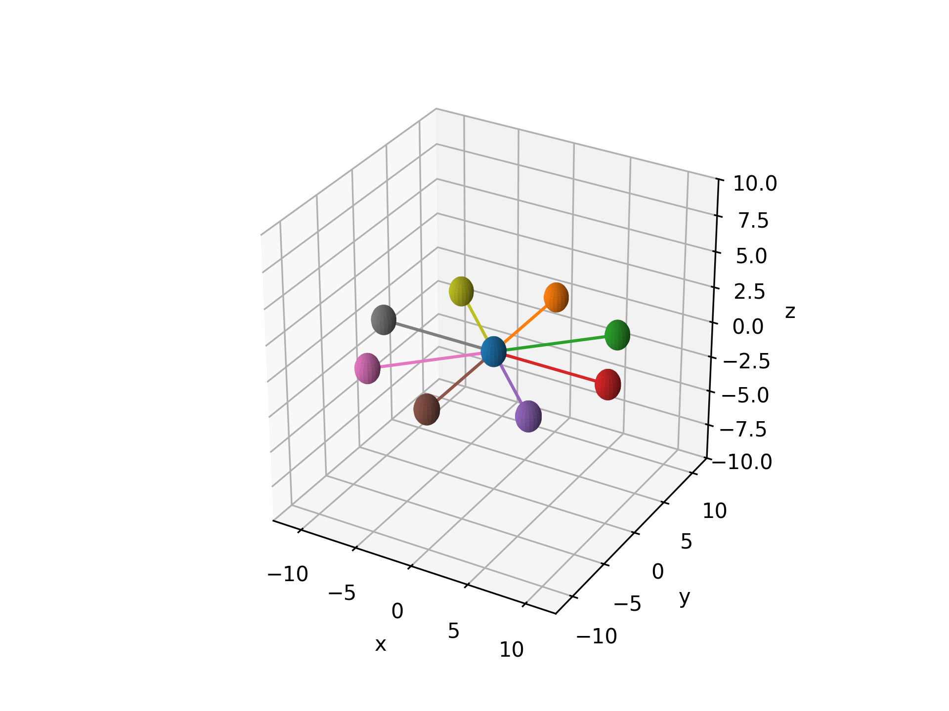
aopy.analysis.base.simulate_ideal_trajectories(targets, origin=[0.0, 0.0, 0.0], resolution=1000)

Simulates straight reach trajectories from a given origin to a list of target points in 3D space. A fixed number of samples is used for each reach (i.e. time to target is constant.)

Parameters:

• targets (numpy.ndarray or list of lists/tuples) – A list or array of target coordinates in space.

• origin (list or tuple, optional) – The origin point from which the trajectories are simulated. Default is zeros in all dimensions.

• resolution (int, optional) – The number of points used to render each trajectory. Default is 1000.

Returns:

An array of simulated trajectories, each being a series of points

from the origin to the corresponding target.

Return type:

(num_targets, resolution, num_dims) numpy.ndarray

Examples

subject = 'MCP015'
entries = db.lookup_mc_sessions(subject=subject)
subjects, ids, dates = db.list_entry_details(entries)
df = aopy.data.tabulate_behavior_data_center_out(preproc_dir, subjects, ids, dates,
                                                metadata=['target_radius', 'session'])
target_radius = df['target_radius'][0]
target_indices = np.unique(df['target_idx'])
target_locations = aopy.data.bmi3d.get_target_locations(preproc_dir, subject,
                                                        te_id, dates[0], target_indices)

ideal_trajectories = simulate_ideal_trajectories(target_locations[1:], target_locations[0])

fig = plt.figure()
ax = fig.add_subplot(111, projection='3d')
aopy.visualization.color_trajectories(ideal_trajectories, target_idx, colors)

aopy.analysis.base.subtract_erp_baseline(erp, time, t0, t1)

Subtract pre-trigger activity from trial-aligned data.

Parameters:

• erp (nt, nch, ntr) – trial-aligned evoked responses

• time (nt) – time axis (in seconds) of the erp, in the same reference frame as t0 and t1

• t0 (float) – start of the baseline window (in seconds)

• t1 (float) – end of the baseline window (in seconds)

Raises:

ValueError – if the baseline window times (t0, t1) are in the wrong order

Returns:

erp after baseline subtraction

Return type:

(nt, nch, ntr)

aopy.analysis.base.windowed_xval_lda_wrapper(data, labels, samplerate, lags=3, nfolds=5, regularization='auto', lda_model=None, return_weights=False, return_confusion_matrix=False)

Perform cross-validation with Linear Discriminant Analysis (LDA) to estimate decoding accuracy at each time point.

This function performs an n-fold cross-validation LDA analysis on time-series data to compute the decoding accuracy across time windows defined by lags. Optionally, it can return the weights of the LDA classifier and/or confusion matrices for each fold.

Parameters:

• data (numpy.ndarray) – The input data array with shape (ntime, nch, ntrials), where ntime is the number of time points, nch is the number of channels, and ntrials is the number of trials.

• labels (numpy.ndarray) – Array of shape (ntrials,) containing the labels for each trial.

• samplerate (float or int) – Samplerate of data. Used to compute the timeaxis.

• lags (int, optional) – The number of time lags to include in the analysis (default is 3). To only use a single timepoint set lags=0

• nfolds (int, optional) – The number of folds for cross-validation (default is 5).

• regularization (str or float, optional) – If regularization should be included when building the LDA model. Input into the shrinkage parameter of the sklearn LDA function. Can either be None, ‘auto’, or a float between 0 and 1.

• lda_model (sklearn LDA class, optional) – User-defined LDA model from sklearn.discriminant_analysis.LinearDiscriminantAnalysis. If None, this function will initialize the model.

• return_weights (bool, optional) – Whether to return the LDA weights (default is False).

• return_confusion_matrix (bool, optional) – Whether to return the confusion matrix for each fold (default is False).

Returns:

Tuple containing:

accuracy (ntime-nlags, nfolds): The decoding accuracy for each time point (and fold if cross-validation is used).

time_axis (nt-nlags): The time-axis for each trial of the output data. When lags>0, each time-point corresponds to the right edge of the window. This is the time point corresponding to the latest data used in decoding.

(Optional) LDA Weights (ntime-lags, nlabels, nfeatures, nfolds): The LDA weights for each time point, channel, and fold if return_weights=True. Note: nfeatures will include lagged features if lags are used.

(Optional) Confusion Matrix (ntime-lags, nlabels, nlabels, nfolds): The confusion matrix for each fold if return_confusion_matrix=True.

Return type:

tuple

Raises:

ValueError – If the input data or labels are not valid, or if there is a mismatch between the data and labels.

Notes

If nfolds < 2, no cross-validation is performed, and the function will calculate the accuracy based on the entire dataset. If nfolds >= 2, k-fold cross-validation is performed, and decoding accuracy is calculated for each fold.

aopy.analysis.base.xval_lda_subsample_wrapper(data, labels, min_trial, cond_mask=None, single_decoding=True, min_unit=None, shuffle_labels=False, nfolds=5, replacement=False, regularization='auto', lda_model=None, return_labels=False, return_weights=False, seed=None)

Perform an n-fold cross-validation with Linear Discriminant Analysis (LDA) using a single unit or multiple units. This functions extracts trials and/or units randomly based on the random seed with/without replacement. The number of trials per target is controlled to be the same across targets You can repeatedly perform this function by changing random seed to estimate the resampling distribution

Parameters:

• data (nunit, ntr) or (nunit, nfeatures, ntr) – neural data. 2 different shapess are allowed.

• labels (ntr) – the labels for each trial.

• min_trial (int) – the minimum number of trials for each label to be extracted if this is 20, 20*(the number of unique labels) trials are extracted

• cond_mask (ntr) – a boolean array. This is a mask to extract trials that satisfies a certain condition (ex. movement onset is more than a certain threshold)

• single_decoding (bool, optional) – If True, LDA is performed using single unit activity separately (default is True)

• min_unit (int, optional) – the number of units used for decoding. This is used only when single_decoding is False. if min_unit is None, decoding is perfomed using all units (default is None)

• shuffle_labels (bool, optional) – whether to shuffle labels or not (default is False)

• nfolds (int, optional) – the number of folds for cross-validation (default is 5)

• replacement (bool, optional) – whether to choose trials with replacement or without replacement

• regularization (str or float, optional) – If regularization should be included when building the LDA model Input into the shrinkage parameter of the sklearn LDA function Can either be None, ‘auto’, or a float between 0 and 1.

• lda_model (sklearn LDA class, optional) – User-defined LDA model from sklearn.discriminant_analysis.LinearDiscriminantAnalysis. If None, this function will initialize the model.

• return_labels (bool, optional) – Whether to return true and predicted labels (default is False).

• return_weights (bool, optional) – Whether to return the LDA weights (default is False).

• seed (int, optional) – random seed

Returns:

Tuple containing:

accuracy (nch) or (float): the decoding accuracy. If single_decoding is False, this gets a single velue.

(Optional) true_Y (nch,ntr) or (ntr): a list of true labels. If single_decoding is False, its shape becomes (ntr).

(Optional) pred_Y (nch,ntr) or (ntr): a list of predicted labels. If single_decoding is False, its shape becomes (ntr).

(Optional) LDA Weights (nlabels,nch,nfolds) or (nlabels,nch,nfeatures,nfolds): The LDA weights if return_weights is True.

Return type:

tuple

Examples

"This is an example of this function using multiprocessing to get a resampling distribution"

import multiprocessing as mp

single_decoding = True
min_unit = None
shuffle_labels = False
n_fold = 5
replacement = False
regularization = 'auto'
lda_model = None
return_labels = True
return_weights = False
n_resample = 100 # the number of resampling
n_processes = 20 # the number of cpus used for the computation

pool = mp.Pool(n_processes)
result_objects = [pool.apply_async(xval_lda_subsample_wrapper,                args=(data, target_idx, min_trials, trial_mask, single_decoding, min_unit, shuffle_labels, n_fold,                     replacement, regularization, lda_model, return_labels, return_weights, ibs)) for ibs in range(n_resample)]
pool.close()

# Organize results
results = [r.get() for r in result_objects]
accuracy, pred_labels_resample, true_labels_resample = zip(*results)
accuracy = np.array(accuracy)
pred_labels_resample = np.array(pred_labels_resample, int)
true_labels_resample = np.array(true_labels_resample, int)

See also

windowed_xval_lda_wrapper()

Behavior

aopy.analysis.behavior.angle_between(v1, v2, in_degrees=False)

Computes the angle between two vectors. By default, the angle will be in radians and fall within the range [0,pi].

Parameters:

• v1 (list or array) – D-dimensional vector

• v2 (list or array) – D-dimensional vector

• in_degrees (bool, optional) – whether to return the angle in units of degrees. Default is False.

Returns:

angle (in radians or degrees)

Return type:

float

aopy.analysis.behavior.calc_segment_duration(events, event_times, start_events, end_events, target_codes=[81, 82, 83, 84, 85, 86, 87, 88], trial_filter=<function <lambda>>)

Calculates the duration of trial segments. Event codes and event times for this function are raw and not trial aligned.

Parameters:

• events (nevents) – events vector, can be codes, event names, anything to match

• event_times (nevents) – time of events in ‘events’

• start_events (int, str, or list, optional) – set of start events to match

• end_events (int, str, or list, optional) – set of end events to match

• target_codes (list, optional) – list of target codes to use for finding targets within trials

• trial_filter (function, optional) – function to apply to each trial’s events to determine whether or not to keep it

Returns:

tuple containing:

segment_duration (list): duration of each segment after filtering

target_codes (list): target index on each segment

Return type:

tuple

aopy.analysis.behavior.calc_success_percent(events, start_events=[b'TARGET_ON'], end_events=[b'REWARD', b'TRIAL_END'], success_events=b'REWARD', window_size=None)

A wrapper around get_trial_segments which counts the number of trials with a reward event and divides by the total number of trials. This function can either calculated the success percent across all trials in the input events, or compute a rolling success percent based on the ‘window_size’ input argument.

See also

calc_success_percent_trials()

Parameters:

• events (nevents) – events vector, can be codes, event names, anything to match

• start_events (int, str, or list, optional) – set of start events to match

• end_events (int, str, or list, optional) – set of end events to match

• success_events (int, str, or list, optional) – which events make a trial a successful trial

• window_size (int, optional) – [in number of trials] For computing rolling success perecent. How many trials to include in each window. If None, this functions calculates the success percent across all trials.

Returns:

success percent = number of successful trials out of all trials attempted.

Return type:

float or array (nwindow)

aopy.analysis.behavior.calc_success_percent_trials(trial_success, window_size=None)

A wrapper around get_trial_segments which counts the number of trials with a reward event and divides by the total number of trials. This function can either calculated the success percent across all trials in the input events, or compute a rolling success percent based on the ‘window_size’ input argument.

See also

calc_success_percent()

Parameters:

• trial_success ((ntrial,) bool array) – boolean array of trials where success is non-zero and failure is zero

• window_size (int, optional) – [in number of trials] For computing rolling success perecent. How many trials to include in each window. If None, this functions calculates the success percent across all trials.

Returns:

success percent = number of successful trials out of all trials attempted.

Return type:

float or array (nwindow)

aopy.analysis.behavior.calc_success_rate(events, event_times, start_events, end_events, success_events, window_size=None)

Calculate the number of successful trials per second with a given trial start and end definition. Inputs are raw event codes and times.

See also

calc_success_rate_trials()

Parameters:

• events (nevents) – events vector, can be codes, event names, anything to match

• event_times (nevents) – time of events in ‘events’

• start_events (int, str, or list, optional) – set of start events to match

• end_events (int, str, or list, optional) – set of end events to match

• success_events (int, str, or list, optional) – which events make a trial a successful trial

• window_size (int, optional) – [ntrials] For computing rolling success perecent. How many trials to include in each window. If None, this functions calculates the success percent across all trials.

Returns:

success rate [success/s] = number of successful trials completed per second of time between the start event(s) and end event(s).

Return type:

float or array (nwindow)

aopy.analysis.behavior.calc_success_rate_trials(trial_success, trial_time, window_size=None)

Calculate the number of successful trials per second with a given trial start and end definition.

See also

calc_success_rate()

Parameters:

• trial_success ((ntrial,) bool array) – boolean array of trials where success is non-zero and failure is zero

• trial_time ((ntrial,) array) – float array of the time taken in each trial (e.g. acquisition time)

• window_size (int, optional) – [ntrials] For computing rolling success perecent. How many trials to include in each window. If None, this functions calculates the success percent across all trials.

Returns:

success rate [success/s] = number of successful trials completed per second of

time between the start event(s) and end event(s).

Return type:

float or array (nwindow)

aopy.analysis.behavior.calc_tracking_error(user_traj, target_traj)

Computes the mean-squared error between the user position and target position over time.

Parameters:

• user_traj (nt,ndim) – user trajectory over a trial segment

• target_traj (nt,ndim) – target trajectory over a trial segment

Returns:

tracking error in each dimension

Return type:

float array (ndim,)

aopy.analysis.behavior.calc_tracking_in_time(event_codes, event_times, proportion=False)

Computes the total amount of time that the cursor is inside the target over a trial segment.

Parameters:

• event_codes (nevents,) – list of event codes

• event_times (nevents,) – list of event times

• proportion (bool, optional) – whether to return the time as a proportion of the total trial segment time. Default is False.

Returns:

amount of time (in seconds) that the cursor was in the target for

Return type:

float

aopy.analysis.behavior.compute_movement_error(trajectory, target_position, rotation_vector=numpy.array, error_axis=1)

Computes movement error of a trajectory relative to the straight line between the origin and a target position.

Parameters:

• trajectory (nt, 2) – The trajectory coordinates for each point in time.

• target_position (2,) – Target position coordinates.

• rotation_vector ((2,) array, optional) – The vector onto which movement will be projected to calculate error. Defaults to np.array([1, 0]).

• error_axis (int, optional) – axis (after rotation) along which to compute the error statistics. Default 1.

Returns:

The error of the trajectory relative to the target position

Return type:

(nt,)

aopy.analysis.behavior.compute_movement_stats(trajectory, target_position, rotation_vector=numpy.array, error_axis=1, return_all_stats=False)

Computes movement statistics of a trajectory relative to a target position.

Parameters:

• trajectory (nt, 2) – The trajectory coordinates for each point in time.

• target_position (2,) – Target position coordinates.

• rotation_vector ((2,) array, optional) – The vector onto which movement will be projected to calculate error. Defaults to np.array([1, 0]).

• error_axis (int, optional) – axis (after rotation) along which to compute the error statistics. Default 1.

Returns:

A tuple containing:

mean (float): The mean error of the trajectory relative to the target position.

std (float): The variance of the error of the trajectory relative to the target position.

auc (float): The area under the curve ofthe trajectory relative to the target position.

additionally, with return_all_stats=True:

abs_mean (float): The mean of the absolute value of the trajectory error.

abs_min (float): The minimum absolute trajectory error.

abs_max (float): The maximum absolute trajectory error.

abs_auc (float): The area under the curve of the absolute value of the trajectory error.

sign (float): 1 if the maximum positive value is bigger than the maximum negative value. -1 otherwise.

signed_min (float): The minimum value if the sign is 1, otherwise the maximum value of the trajectory error.

signed_max (float): The maximum value if the sign is 1, otherwise the minimum value of the trajectory error.

signed_abs_mean (float): The sign multiplied by the absolute value of the mean trajectory error.

Return type:

tuple

aopy.analysis.behavior.compute_path_length_per_trajectory(trajectory)

This function calculates the path length by computing the distance from all points for a single trajectory. The input trajectry could be cursor or eye trajectory from a single trial. It returns a single value for path length.

Parameters:

trajectory (nt x 2) – single trial trajectory, could be a cursor trajectory or eye trajectory

Returns:

length of the trajectory

Return type:

path_length (float)

aopy.analysis.behavior.correlate_trajectories(trajectories, center=True, verbose=False)

Correlates multiple trajectory datasets across trials by computing the Pearson correlation coefficient (R) between all pairs of trials. This function computs R for each trajectory dimension, then returns a weighted average based on the variance.

Parameters:

• trajectories (nt, ndim, ntrials) – Trajectories to correlate, where nt is the number of timepoints, ntrials is the number of trials, and ndims is the number of dimensions for each trajectory (i.e. x, y, z).

• center (bool) – If each trial should be centered before computing correlation. (Safaie et al. 2023 sets this to true)

• verbose (bool) – If True, prints a progress bar during computation via the tqdm module.

Returns:

A 2D numpy array of Pearson correlation (R) scores between each pair of trials.

The shape of the output will be (ntrials, ntrials).

Return type:

ndarray

aopy.analysis.behavior.get_cursor_leave_time(cursor_traj, samplerate, target_radius, cursor_radius=0)

Compute the times when the cursor leaves the center target radius

Parameters:

• cursor_traj ((ntr,) np object array) – cursor trajectory that begins with the time when the cursor enters the center target

• fs (float) – sampling rate in Hz

• target_radius (float) – the radius of the center target in cm

• cursor_radius (float) – the radius of the cursor in cm. Default is 0

Returns:

cursor leave times relative to the time when the cursor enters the center target

Return type:

cursor_leave_time (ntr)

aopy.analysis.behavior.get_movement_onset(cursor_traj, fs, trial_start, target_onset, gocue, numsd=3.0, butter_order=4, low_cut=20, thr=None)

Compute movement onset when cursor speed crosses threshold based on mean and standard deviation in baseline period. Speed is estimated from cursor trajectories and low-pass filtered to remove noise. Baseline is defined as the period between target onset and gocue because speed still exists soon after the cursor enters the center target.

Parameters:

• cursor_traj ((ntr,) np object array) – cursor trajectory that begins with the time when the cursor enters the center target

• fs (float) – sampling rate in Hz

• trial_start (ntr) – trial start time (the time when the cursor enters the center target) relative to experiment start time in sec

• target_onset (ntr) – target onset relative to experiment start time in sec

• gocue (ntr) – gocue (the time when the center target disappears) relative to experiment start time in sec

• numsd (float) – for determining threshold at each trial

• butter_order (int) – the order for the butterworth filter

• low_cut (float) – cut off frequency for low pass filter in Hz

• thr (float) – thr when you want to use constant threshold across trials. If thr=None, thr is computed by mean + numsd*std in the period from target onset to gocue.

Returns:

movement onset relative to trial start time (the time when the cursor enters the center target) in sec

Return type:

movement_onset (ntr)

aopy.analysis.behavior.time_to_target(event_codes, event_times, target_codes=[81, 82, 83, 84, 85, 86, 87, 88], go_cue_code=32, reward_code=48)

This function calculates reach time to target only on rewarded trials given trial aligned event codes and event times See: aopy.preproc.base.get_trial_segments_and_times() .

Note

Trials are filtered to only include rewarded trials so that all trials have the same length.

Parameters:

• event_codes (list) – trial aligned event codes

• event_times (list) – trial aligned event times corresponding to the event codes. These event codes and event times could be the output of preproc.base.get_trial_segments_and_times()

• target_codes (list) – list of event codes for cursor entering peripheral target

• go_cue_code (int) – event code for go cue

• reward_code (int) – event code for reward

Returns:

tuple containing:

reachtime_pertarget (list): duration of each segment after filtering

trial_id (list): target index on each segment

Return type:

tuple

aopy.analysis.behavior.unit_vector(vector)

Finds the unit vector of a given vector.

Parameters:

vector (list or array) – D-dimensional vector

Returns:

D-dimensional vector with a magnitude of 1

Return type:

unit_vector (list or array)

aopy.analysis.behavior.vector_angle(vector, in_degrees=False)

Computes the angle of a vector on the unit circle.

Parameters:

• vector (list or array) – D-dimensional vector

• in_degrees (bool, optional) – whether to return the angle in units of degrees. Default is False.

Returns:

angle (in radians or degrees)

Return type:

float

CellType

aopy.analysis.celltype.classify_cells_spike_width(waveform_data, samplerate, std_threshold=3, pca_varthresh=0.75, min_wfs=10)

Calculates waveform width and classifies units into putative exciatory and inhibitory cell types based on pulse width. Units with lower spike width are considered inhibitory cells (label: 0) and higher spike width are considered excitatory cells (label: 1) The pulse width is defined as the time between the waveform trough to the waveform peak. (trough-to-peak time) Assumes all waveforms are recorded for the same number of time points.

This function conducts the following processing steps:

**1. ** For each unit, project each waveform into the top PCs. Number of PCs determined by ‘pca_varthresh’

**2. ** For each unit, remove outlier spikes. Outlier threhsold determined by ‘std_threshold’. If the number of waveforms is less than ‘min_wf’, no waveforms are removed.

**3. ** For each unit, average remaining waveforms.

**4. ** For each unit, calculate spike width using a local polynomial interpolation.

**5. ** Use a gaussian mixture model to classify all units

Parameters:

• waveform_data (nunit long list of (nt x nwaveforms) arrays) – Waveforms of each unit. Each element of the list is a 2D array for each unit. Each 2D array contains the timeseries of all recorded waveforms for a given unit.

• samplerate (float) – sampling rate of the points in each waveform.

• std_threshold (float) – For outlier removal. The maximum number of standard deviations (in PC space) away from the mean a given waveform is allowed to be. Defaults to 3

• pca_varthresh (float) – Variance threshold for determining the number of dimensions to project spiking data onto. Defaults to 0.75.

• min_wfs (int) – Minimum number of waveform samples required to perform outlier detection.

Returns:

A tuple containing

TTP (nunit): Spike width of each unit. [us]

unit_labels (nunit): Label of each unit. 0: low spike width (inhibitory), 1: high spike width (excitatory)

avg_wfs (nunit, nt): Average waveform of accepted waveforms for each unit

sss_unitid (1D):* Unit index of spikes with a lower number of spikes than allowed by ‘min_wfs’

Return type:

tuple

aopy.analysis.celltype.find_trough_peak_idx(unit_data)

This function calculates the trough-to-peak time at the index level (0th order) by finding the minimum value of the waveform, and identifying that as the trough index. To calculate the peak index, this function finds the index corresponding to the first negative derivative of the waveform. If there is no next negative derivative of the waveform, this function returns the last index as the peak time.

Parameters:

unit_data (nt, nch) – Array of waveforms (Can be a 1D array with dimension nt)

Returns:

A tuple containing

troughidx (nch): Array of indices corresponding to the trough time for each channel

peakidx (nch): Array of indices corresponding ot the peak time for each channel.

Return type:

tuple

aopy.analysis.celltype.get_unit_spiking_mean_variance(spiking_data)

This function calculates the mean spiking count and the spiking count variance in spiking data across trials for each unit.

Parameters:

spiking_data (ntime, nunits, ntr) – Input spiking data

Returns:

A tuple containing

unit_mean: The mean spike counts for each unit across the input time

unit_variance: The spike count variance for each unit across the input time

Return type:

Tuple

Tuning

aopy.analysis.tuning.calc_dprime(*dist)

d-prime or the sensitivity index is the peak-to-peak difference of means of the signals across categories divided by their pooled (mean) standard deviation. The formula is as follows:

\[d' = \frac{µ_{max} - µ_{min}}{\sqrt{\sum_{i=0}^{n-1} (p_i)\sigma_i^2}}\]

where \(µ_{max} - µ_{min}\) is the peak-to-peak distance across category means, \(p_i\) is the proportion of trials in the i-th category, and \(\sigma_i^2\) is the standard deviation of the i-th category.

Parameters:

*dist (ntr, nch) – distribution of the data for each category. d-prime is calculated along the first axis.

Returns:

d-prime value for each channel or unit.

Return type:

(nch)

Examples

\(d'\) is essentially a signal-to-noise ratio. In the simple case of two distributions, the numerator is the distance between the two means while the denominator is the average noise within each distribution. If the distributions are normal and of equal variance then the \(d'\) value becomes the z-score of the difference between the two means.

noise_dist = np.array([[0, 1], [0, 1], [0, 1]]).T
signal_dist = np.array([[0.5, 1.5], [1, 2], [1.5, 2.5]]).T
dprime = aopy.analysis.calc_dprime(noise_dist, signal_dist)
print(dprime)
>>> np.array([1, 2, 3])

If there are more than two classes, d-prime finds the maximum signal-to-noise ratio, as illustrated in this pictorial from Williams, J. J. (2013). The numerator (peak-to-peak distance between distributions) approximates the “signal” while the denominator (pooled standard deviation of each distribution) approximates the “noise”.

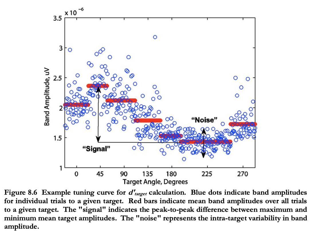
Another simple example with 3 distributions:

dist_1 = np.array([0, 1])
dist_2 = np.array([1, 2])
dist_3 = np.array([2, 3])
dprime = aopy.analysis.calc_dprime(dist_1, dist_2, dist_3)
print(dprime)
>>> 4.

aopy.analysis.tuning.convert_target_to_direction(target_locations, origin=[0, 0], zero_axis=[0, 1], clockwise=True)

Converts target index to target direction in radians. NaNs are returned for targets at the origin.

Parameters:

• target_locations (ntargets, 2) – array of unique target (x, y) locations

• origin (2-tuple) – (x,y) coordinate of the center of all targets defining the polar plane. Default is [0,0].

• zero_axis (2-tuple) – (x,y) coordinate of the axis representing zero degrees. Default is [0,1] (up).

• clockwise (bool) – direction of rotation. Default True.

Returns:

target direction in radians for each trial

Return type:

(ntarget,) array

aopy.analysis.tuning.curve_fitting_func(target_theta, b1, b2, b3)

Parameters:

• target_theta (float) – center out task target direction index [degrees]

• b1 (float) – parameters used for curve fitting

• b2 (float) – parameters used for curve fitting

• b3 (float) – parameters used for curve fitting

\[b1 * cos(\theta) + b2 * sin(\theta) + b3\]

Returns:

Evaluation of the fitting function for a given target.

Return type:

float

aopy.analysis.tuning.get_mean_fr_per_condition(data, condition_labels, return_significance=False)

This function computes the average activity for each feature and trial.

Parameters:

• data (nt, nch, ntrials) – Trial aligned neural data

• condition_labels (ntrials) – condition label for each trial

• return_significance (bool) – Uses the one-way ANOVA test to compute a p-value for each channel/unit

Returns:

Tuple containing:

means_d (nch, nconditions): = mean firing rate per neuron per target direction

stds_d (nch, nconditions): standard deviation from mean firing rate per neuron

pvalue (nch, optional): significance of modulation

Return type:

tuple

aopy.analysis.tuning.get_modulation_depth(b1, b2)

Calculates modulation depth from curve fitting parameters as follows:

\[\sqrt{b_1^2+b_2^2}\]

Returns:

Modulation depth (amplitude) of the curve fit

Return type:

float

aopy.analysis.tuning.get_per_target_response(data, target_idx)

Organizes trial response per target. Pads with nans if there are unequal number of trials per target.

Parameters:

• data (nt, nch, ntrials) – trial aligned neural data

• target_idx (ntrials) – target index for each trial

Returns:

Tuple containing:

per_target_response (ntargets, nt, nch, ntrials/ntargets): trial aligned neural data per target

unique_targets (ntargets): unique target indices corresponding to the 3rd dimension of per_target_response

Return type:

tuple

Examples

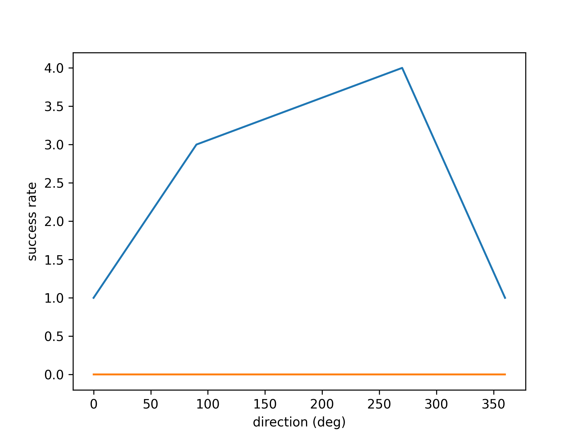
aopy.analysis.tuning.get_preferred_direction(b1, b2)

Calculates preferred direction from curve fitting parameters as follows:

\[arctan(\frac{b_1^2}{b_2^2})\]

Returns:

Preferred direction of the curve fit in radians

Return type:

float

aopy.analysis.tuning.run_tuningcurve_fit(mean_fr, targets, fit_with_nans=False, min_data_pts=3)

This function calculates the tuning parameters from center out task neural data. It fits a sinusoidal tuning curve to the mean firing rates for each unit. Uses approach outlined in Orsborn 2014/Georgopolous 1986. Note: To orient PDs with the quadrant of best fit, this function samples the target location with high resolution between 0-360 degrees.

Parameters:

• mean_fr (nunits, ntargets) – The average firing rate for each unit for each target.

• targets (ntargets) – Targets locations to fit to [Degrees]. Corresponds to order of targets in ‘mean_fr’ (Xaxis in the fit). Targets should be monotonically increasing.

• fit_with_nans (bool) – Optional. Control if the curve fitting should be performed for a unit in the presence of nans. If true curve fitting will be run on non-nan values but will return nan is less than 3 non-nan values. If false, any unit that contains a nan will have the corresponding outputs set to nan.

• min_data_pts (int) – Optional.

Returns:

Tuple containing:

fit_params (3, nunits): Curve fitting parameters for each unit

modulation depth (ntargets, nunits): Modulation depth of each unit

preferred direction (ntargets, nunits): preferred direction of each unit [rad]

Return type:

tuple

KFDecoder

class aopy.analysis.kfdecoder.KFDecoder(C=1)

Kalman Filter Decoder

Parameters:

C (float, optional) – default 1 This parameter scales the noise matrix associated with the transition in kinematic states. It effectively allows changing the weight of the new neural evidence in the current update. Our implementation of the Kalman filter for neural decoding is based on that of Wu et al 2003 (https://papers.nips.cc/paper/2178-neural-decoding-of-cursor-motion-using-a-kalman-filter.pdf) with the exception of the addition of the parameter C. The original implementation has previously been coded in Matlab by Dan Morris (http://dmorris.net/projects/neural_decoding.html#code)

model

list of matrices: | [State Transition model, | Covariance of State Transition model, | Observation model, | Covariance of Observation model]

Type:

[A, W, H, Q] list

fit(X_kf_train, y_train)

Train Kalman Filter Decoder

Parameters:

• X_kf_train (ntime , nfeatures) – This is the neural data in Kalman filter format. See example file for an example of how to format the neural data correctly.

• y_train (ntime , noutputs) – These are the outputs that are being predicted

Calculations for \(A\), \(W\), \(H\), \(Q\) are as follows:

\[A = X2*X1' (X1*X1')^{-1}\]

\[W = \frac{(X_2 - A*X_1)(X_2 - A*X_1)'}{(timepoints - 1)}\]

\[H = Y*X'(X*X')^{-1}\]

\[Q = \frac{(Y-HX)(Y-HX)' }{time points}\]

fit_awf(X_kf_train, y_train, A, W)

Train Kalman Filter Decoder with A and W fixed. A is the state transition model and W is the associated covariance

Parameters:

• X_kf_train (ntime , nfeatures) – This is the neural data in Kalman filter format. See example file for an example of how to format the neural data correctly

• y_train (ntime , noutputs) – These are the outputs that are being predicted

Calculations as follows:

\[H = Y*X'(X*X')^{-1}\]

\[Q = \frac{(Y-HX)(Y-HX)' }{time points}\]

predict(X_kf_test, y_test)

Predict outcomes using trained Kalman Filter Decoder

Args: X_kf_test (ntime, nfeatures): This is the neural data in Kalman filter format. y_test (ntime , noutputs): The actual outputs. This parameter is necesary for the Kalman filter (unlike other decoders) because the first value is nececessary for initialization

Returns:

The predicted outputs

Return type:

y_test_predicted (ntime, noutputs)

Latency

Code for determining the latency of responses to stimulation

AccLLR is based on the paper:

Banerjee A, Dean HL, Pesaran B. A likelihood method for computing selection times in spiking and local field potential activity. J Neurophysiol. 2010 Dec;104(6):3705-20. doi: 10.1152/jn.00036.2010. Epub 2010 Sep 8. https://pubmed.ncbi.nlm.nih.gov/20884767/

Main function: calc_accllr_st()

aopy.analysis.latency.calc_accllr_lfp(lfp_altcond, lfp_nullcond, lfp_altcond_lowpass, lfp_nullcond_lowpass, common_variance=True)

Accumulated log likelihood for single channel LFP data.

Note

As quoted from Banerjee et al. (2010), the common_variance parameter should be set to True: “Since AccLLR changes for LFP activity are scaled by the noise variance for each condition, if the noise variances for each condition differ, the AccLLRs scale differently and this leads to the need for different upper and lower bounds at the discrimination stage. To allow the simplicity of using the same bound for both conditions (see the following subsection), we assume that the variance of activity under each condition is the same.”

Note

Unsure whether the lowpass filtered version of the lfp should be used in place of the lfp entirely. That is how the Pesaran lab code works, however it doesn’t seem to make sense to throw away the raw lfp, so here I use the lowpass filtered version for the mean estimate across trials but use the raw lfp for single trials.

Note

Finally, there is a difference between how the cumulative sum is calculated here versus in the Pesaran lab code. Here we include the first value of the LLR as the first value of the accLLR. However, the Pesaran lab truncates the accLLR so that it starts at the second sum.

Parameters:

• lfp_altcond ((nt, ntrial) array) – lfp data for alternative condition trials

• lfp_nullcond ((nt, ntrial) array) – lfp data for null condition trials. The number of null condition trials must be the same as the number of alternative condition trials.

• lfp_altcond_lowpass ((nt, ntrial) array) – low-pass filtered copy of alternative condition trials. If desired, just pass the lfp_altcond again to avoid using a low-pass filtered version for model building.

• lfp_nullcond_lowpass ((nt, ntrial) array) – low-pass filtered copy of null condition trials

• common_variance (bool, optional) – calculate a shared variance of event and null lfp (see notes). Default True.

Returns:

tuple containing:

accllr_altcond ((nt, ntrial) array): accumulated log-likelihood for alterative condition trials

accllr_nullcond ((nt, ntrial) array): accumulated log-likelihood for null condition trials

Return type:

tuple

aopy.analysis.latency.calc_accllr_performance(accllr_altcond, accllr_nullcond, nlevels=200)

Calculate the probabilities and selection times of accllr trials for a number of different levels, evenly spaced between 0 and the max value of the accllr series.

Parameters:

• event_accllr (nt, ntrial) – accllr timeseries for alternative condition trials

• null_accllr (nt, ntrial) – accllr timeseries for null condition trials

• nlevels (int, optional) – number of levels to calculate. Defaults to 200.

Returns:

tuple containing:

p_altcond (nlevels,3): probability of upper, lower, and unknown level detections for the alternative condition at each detection level

p_nullcond (nlevels,3): probability of upper, lower, and unknown level detections for the null condition at each detection level

selection_idx (nlevels): index at which accllr crosses upper threshold (or nan if missed) for each trial, averaged across trials

levels (nlevels): levels used for calculation of probabilities

Return type:

tuple

aopy.analysis.latency.calc_accllr_roc(accllr_altcond, accllr_nullcond)

ROC analysis on accllr data. Groups the data according to class (alt or null) and computes area under the curve (AUC) using the DeLong method.

Parameters:

• accllr_altcond ((ntrial,) array) – a single accumulated llr across trials for alternative condition trials. Usually we pick the end of the accumulation window as the timepoint of interest.

• accllr_nullcond ((ntrial,) array) – a single accumulated llr across trials for null condition trials.

Returns:

tuple containing:

auc (float): area under the curve

se (float): error across trials of the auc

Return type:

tuple

aopy.analysis.latency.calc_accllr_st(data_altcond, data_nullcond, lowpass_altcond, lowpass_nullcond, modality, bin_width, nlevels=None, match_selectivity=False, match_ch=None, noise_sd_step=1, parallel=True, verbose=True)

Calculate accllr selection time for a multiple channels with optional selectivity matching. Selectivity is defined by the area under the ROC curve. To match selectivity, we add gaussian noise to channel until selectivity is constant across all channels.

Based on the paper:

Banerjee A, Dean HL, Pesaran B. A likelihood method for computing selection times in spiking and local field potential activity. J Neurophysiol. 2010 Dec;104(6):3705-20. doi: 10.1152/jn.00036.2010. Epub 2010 Sep 8. https://pubmed.ncbi.nlm.nih.gov/20884767/

Note

No noise is added to the models built on the lowpass versions of data. It is unclear how this step was performed in the original paper.

Parameters:

• data_altcond ((nt, nch, ntrial)) – lfp channel data for trials from the alternative condition

• data_nullcond ((nt, nch, ntrial)) – lfp channel data for trials from the null condition

• lowpass_altcond ((nt, nch, ntrial) array) – low-pass filtered copy of alternative condition trials. If desired, just pass the lfp_altcond again to avoid using a low-pass filtered version for model building.

• lowpass_nullcond ((nt, nch, ntrial) array) – low-pass filtered copy of null condition trials

• modality (str) – type of data being inputted (“lfp”, “spikes”, etc.)

• bin_width (float) – bin width of input activity, or 1./samplerate for lfp data

• nlevels (int) – number of levels at which to test accllr performance

• match_selectivity (bool, optional) – if True, add noise to input data to match selectivity across channels. Default False.

• match_ch ((nch,) bool array or None, optional) – if set, limit selectivity matching to only these channels. Default None.

• noise_sd_step (float, optional) – standard deviation step size to take when adding noise to ch data. Default 1.

• parallel (bool or mp.pool.Pool) – whether to use parallel processing. Can optionally be a pool object to use an existing pool. If True, a new pool is created with the number of CPUs available. If False, computation is done serially across channels.

• verbose (bool, optional) – Print progress. Defaults to True.

Returns:

tuple containing:

selection_time (nch, ntrials): time (in s) at which each trial

roc_auc (nch,): area under the curve from receiver operating characteristic analysis

roc_se (nch,): error across trials of the auc analysis

roc_p_fdrc (nch,): p-value for each channel after false-discovery-rate correction

Return type:

tuple

Examples

Below are powers in 50-250hz band of three channels of laser-evoked response in motor cortex, aligned to laser onset across 350 trials, 50 ms before and after. We first apply AccLLR without selectivity matching:

st, roc_auc, roc_se, roc_p_fdrc = accllr.calc_accllr_st(altcond, nullcond, altcond,
                                                        nullcond, 'lfp', 1./samplerate)
accllr_mean = np.nanmean(st, axis=1)

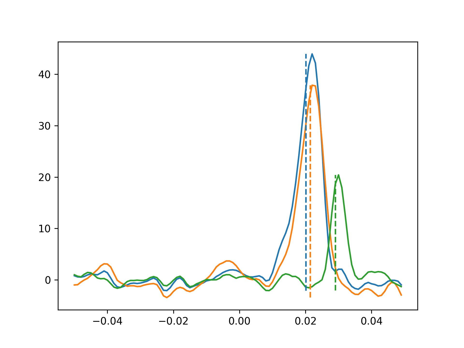
The dotted lines are the estimated selection times returned by accllr. Note that the bigger responses have faster selection times – to test whether the estimates are biased by the larger peaks being easier to identify, we can add noise until they match the selectivity of the smaller peak. Selectivity is defined by ROC analysis – our ability to discriminate between laser event trials and null trials.

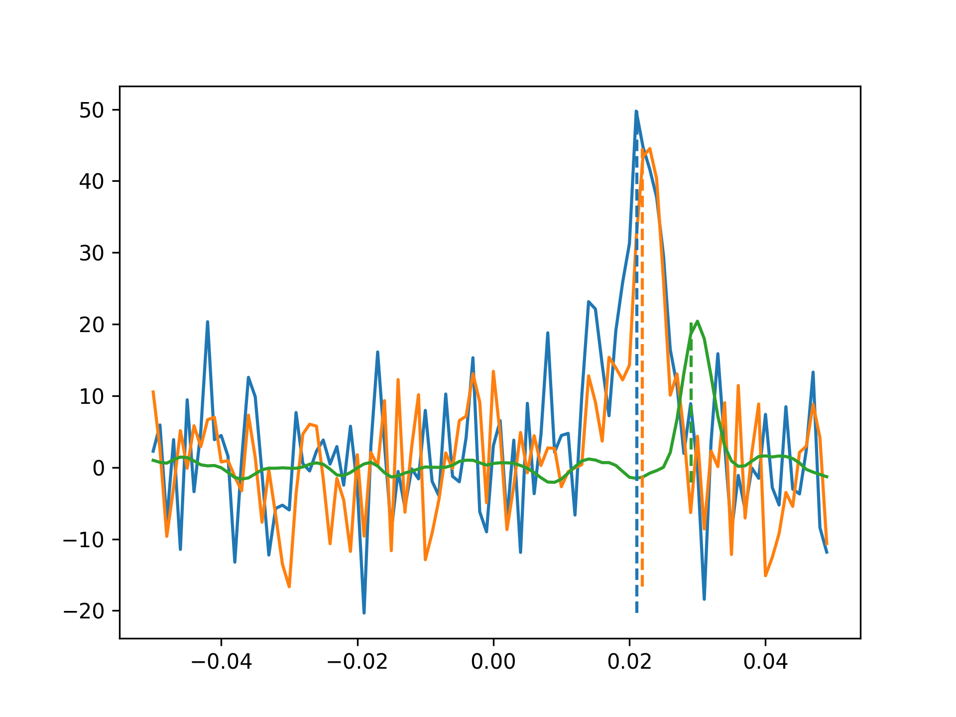
Note that the selection times for the two larger peaks have shifted slightly to the right, but are still earlier than the smaller peak, despite having the same (or lower) selectivity. Thus, we can be confident that the bigger peaks appear faster than the smaller one.

aopy.analysis.latency.calc_accllr_st_single_ch(data_altcond_ch, data_nullcond_ch, lowpass_altcond_ch, lowpass_nullcond_ch, modality, bin_width, nlevels, verbose_out=False)

Calculate accllr selection time for a single channel

Parameters:

• data_altcond_ch ((nt, ntrial)) – lfp data for trials from the alternative condition

• data_nullcond_ch ((nt, ntrial)) – lfp data for trials from the null condition

• lowpass_altcond_ch ((nt, ntrial) array) – low-pass filtered copy of alternative condition trials. If desired, just pass the lfp_altcond again to avoid using a low-pass filtered version for model building.

• lowpass_nullcond_ch ((nt, ntrial) array) – low-pass filtered copy of null condition trials

• modality (str) – type of data being inputted (“lfp”, “spikes”, etc.)

• bin_width (float) – bin width of input activity, or 1./samplerate for lfp data

• nlevels (int) – number of levels at which to test accllr performance

• verbose_out (bool, optional) – Include probabilities of detection and accllr in the output. Defaults to False.

Returns:

tuple containing:

selection_time (nch, ntrials): time (in s) at which each trial

roc_auc (nch,): area under the curve from receiver operating characteristic analysis

roc_se (nch,): error across trials of the auc analysis

Return type:

tuple

aopy.analysis.latency.calc_delong_roc_variance(ground_truth, predictions)

Computes ROC AUC variance for a single set of predictions using the fast version of DeLong’s method for computing the covariance of unadjusted AUC.

Adapted from https://github.com/Netflix/vmaf/

Parameters:

• ground_truth (nt) – array of 0 and 1 ground truth classes

• predictions (nt) – array of floats of the probability of being class 1

Returns:

tuple containing:

auc (float): area under the curve after ROC analysis

cov (float): variance of the predicted auc

Return type:

tuple

Reference:

@article{sun2014fast,

title={Fast Implementation of DeLong’s Algorithm for

Comparing the Areas Under Correlated Receiver Oerating Characteristic Curves},

author={Xu Sun and Weichao Xu}, journal={IEEE Signal Processing Letters}, volume={21}, number={11}, pages={1389–1393}, year={2014}, publisher={IEEE}

}

aopy.analysis.latency.calc_llr_gauss(lfp, lfp_mean_1, lfp_mean_2, lfp_sigma_1, lfp_sigma_2)

Calculate log likelihood ratio of lfp data belonging to one of two gaussian models with no history.

Parameters:

• lfp ((nt,) array) – single trial lfp data

• lfp_mean_1 ((nt,) array) – mean across trials of lfp data from condition 1

• lfp_mean_2 ((nt,) array) – mean across trials of lfp data from condition 2

• lfp_sigma_1 (float) – variance of lfp data from condition 1

• lfp_sigma_2 (float) – variance of lfp data from condition 2

Returns:

log likelihood ratio

Return type:

(nt,) array

aopy.analysis.latency.choose_best_level(p_altcond, p_nullcond, levels)

Given a list of probabilities for upper, lower, and unknown detections at various levels, select the level with the highest difference in correct detection and incorrect detection.

Parameters:

• p_altcond ((ntrial, 3) array) – [upper, lower, unknown] detections for trials from the alternative condition

• p_nullcond ((ntrial, 3) array) – [upper, lower, unknown] detections for trials from the null condition

• levels (nlevels) – levels used for calculation of probabilities

Returns:

the best level to use

Return type:

float

aopy.analysis.latency.compute_midrank(x)

Computes midranks.

Adapted from: https://github.com/yandexdataschool/roc_comparison

Parameters:

x (npt) – data to compute midrank over

Returns:

array of midranks

Return type:

(npt)

aopy.analysis.latency.detect_accllr(accllr, upper, lower)

Calculate the probability of upper, lower, and unknown level detections. This version is present only for readability, since it is very slow. See detect_accllr_fast().

Parameters:

• accllr (nt, ntrial) – the accllr timeseries to test across trials

• upper (float) – upper level

• lower (float) – lower level

Returns:

tuple containing:

p (3,): probability of upper, lower, and unknown level detections

selection_idx (ntrial): index at which accllr crosses upper threshold (or nan if missed) for each trial

Return type:

tuple

aopy.analysis.latency.detect_accllr_fast(accllr, upper, lower)

Calculate the probability of upper, lower, and unknown level detections. This faster algorithm avoids looping over every single trial, greatly speeding up computations of accllr.

Parameters:

• accllr (nt, ntrial) – the accllr timeseries to test across trials

• upper (float) – upper level

• lower (float) – lower level

Returns:

tuple containing:

p (3,): probability of upper, lower, and unknown level detections

selection_idx (ntrial): index at which accllr crosses upper threshold (or nan if missed) for each trial

Return type:

tuple

aopy.analysis.latency.detect_erp_response(nullcond, altcond, samplerate, num_sd=3, debug=False)

Calculates the latency with which an ERP becomes maximized. Also checks for significant responses using a threshold of num_sd standard deviations above the mean of a null condition (e.g. baseline) response across time. Can be used on single trial or trial-averaged ERP data.

Parameters:

• nullcond (nt, nch, ntr) – responses for null condition trials

• altcond (nt, nch, ntr) – responses for alternative condition trials

• samplerate (float) – sampling rate of the data

• num_sd (float, optional) – number of standard deviations to use as a threshold for significant response. Default 3.

• debug (bool, optional) – if True, plot the data and computed thresholds. Default False.

Returns:

array of latencies in seconds for each channel. NaN indicates no response above threshold.

Return type:

(nch, ntr)

Examples

Make a null baseline and an alternate condition response that are both uniform random noise. Then add a linearly increasing signal to one channel in the alternate condition response. The other channel will have no signal.

fs = 100
nt = fs * 2
nch = 2
ntr = 10
null_data = np.random.uniform(-1, 1, (nt, nch, ntr))
alt_data = np.random.uniform(-1, 1, (nt, nch, ntr))
alt_data[:,1,:] += np.tile(np.expand_dims(np.arange(nt)/10, 1), (1,ntr))

latency = aopy.analysis.latency.detect_erp_response(null_data, alt_data, fs, 3, debug=True)
self.assertEqual(latency.shape, (nch, ntr))

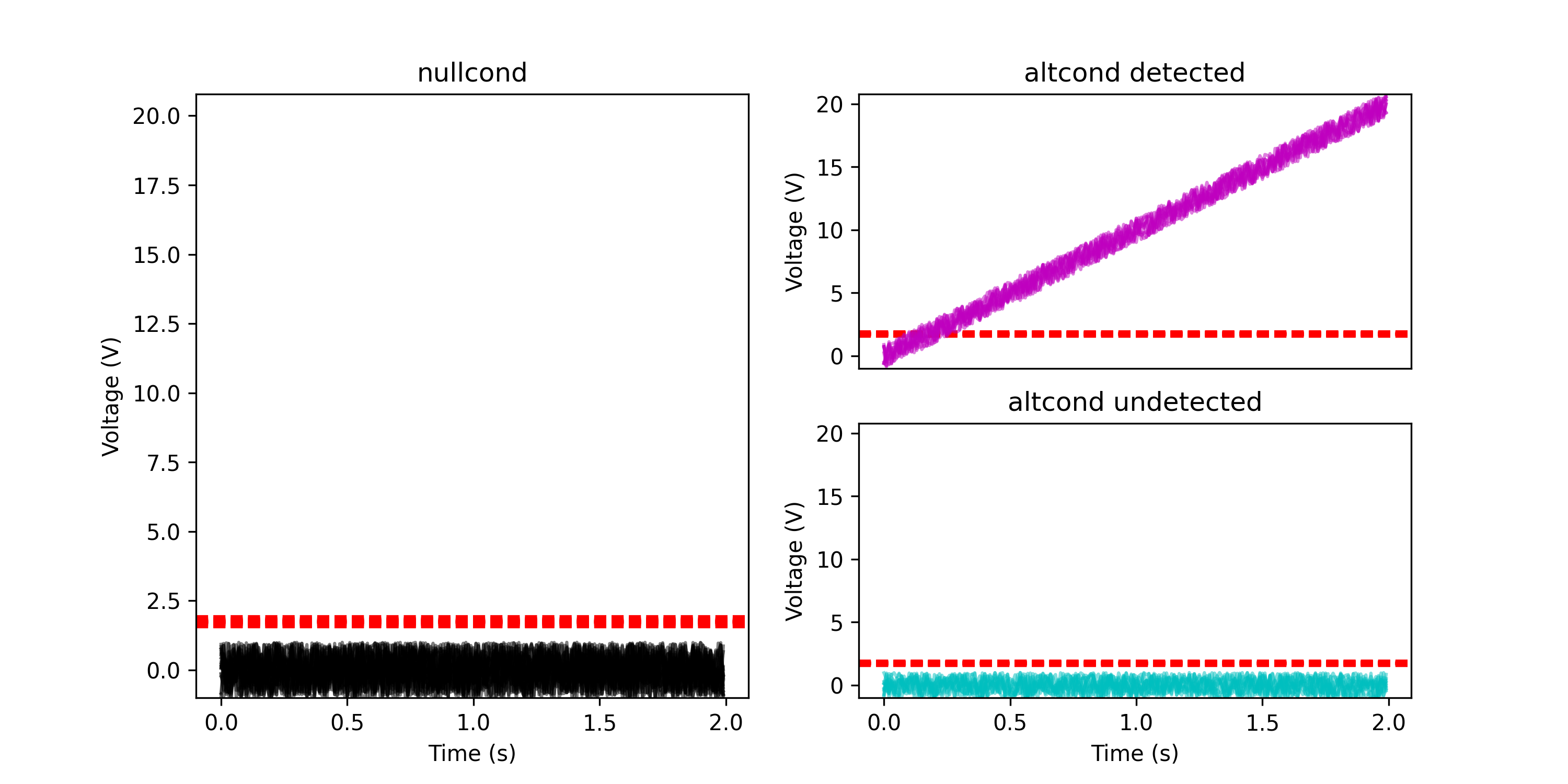
aopy.analysis.latency.detect_itpc_response(im_nullcond, im_altcond, samplerate, num_sd=3, debug=False)

Calculates the latency with which itpc becomes maximized for the given analytical signals. Also checks for significant responses using a threshold of num_sd standard deviations above the mean of a null condition (e.g. baseline) response.

Parameters:

• im_nullcond (nt, nch, ntrial) – analytical signals for null condition trials

• im_altcond (nt, nch, ntrial) – analytical signals for alternative condition trials

• samplerate (float) – sampling rate of the data

• num_sd (float, optional) – number of standard deviations to use as a threshold for significant response. Default 3.

• debug (bool, optional) – if True, plot the itpc values and computed thresholds. Default False.

Returns:

array of latencies in seconds for each channel. NaN indicates no response above threshold.

Return type:

nch

Examples

Create a null baseline and an alternate condition response that are both uniform random noise. Then add a sinusoidal signal to the alternate condition response. On one channel the signal is amplitude 1 (smaller than noise) and on the other channel it is amplitude 10 (bigger than noise).

fs = 100
nt = fs * 2
nch = 2
ntr = 10
null_data = np.random.uniform(-1, 1, (nt, nch, ntr))
alt_data = np.random.uniform(-1, 1, (nt, nch, ntr))
alt_data[:,0,:] += np.tile(np.expand_dims(np.sin(np.arange(nt)*np.pi/10), 1), (1,ntr))
alt_data[:,1,:] += np.tile(np.expand_dims(10*np.sin(np.arange(nt)*np.pi/10), 1), (1,ntr))

im_nullcond = signal.hilbert(null_data, axis=0)
im_altcond = signal.hilbert(alt_data, axis=0)

latency = aopy.analysis.latency.detect_itpc_response(im_nullcond, im_altcond, fs, 5, debug=True)

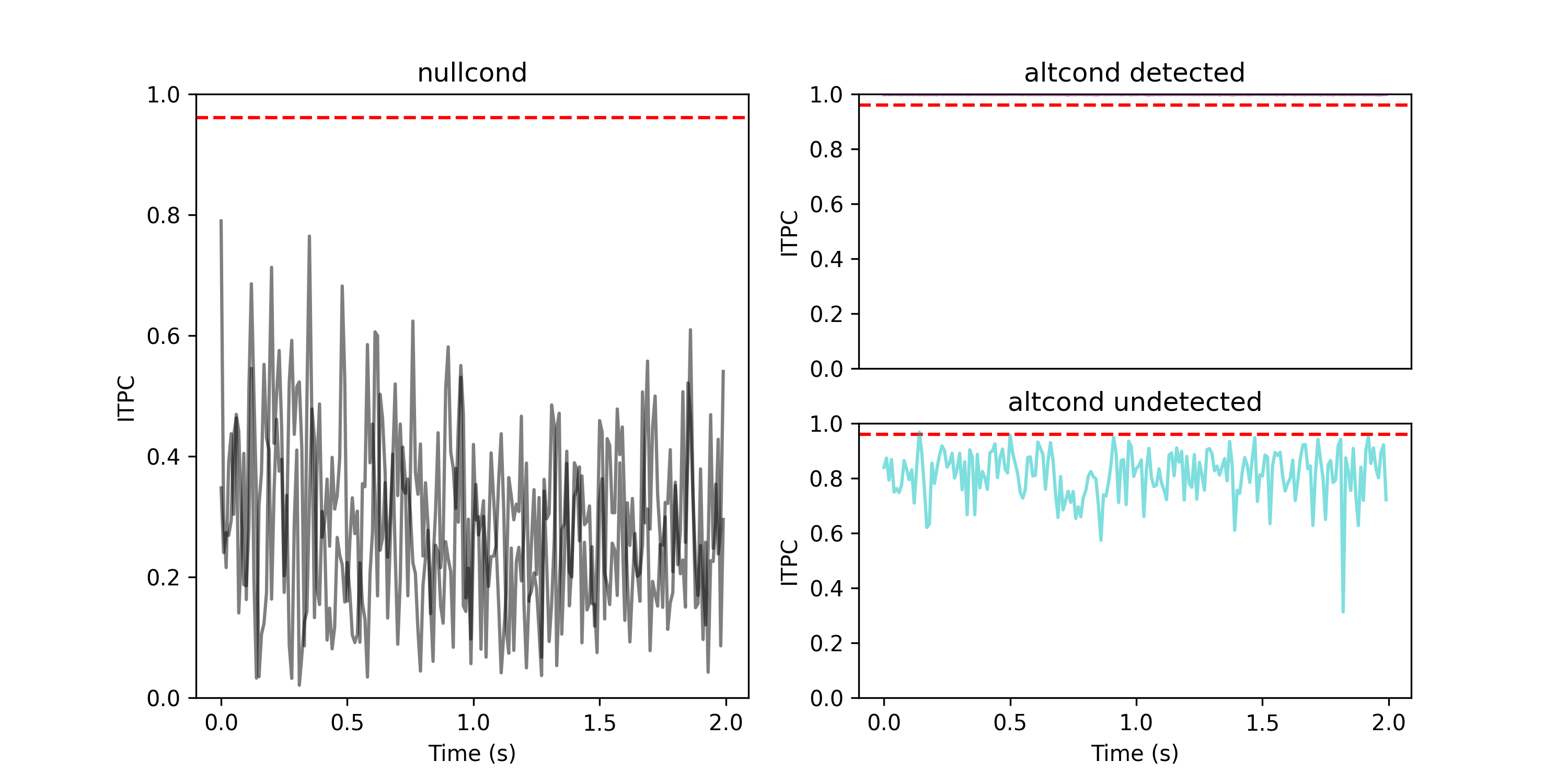
aopy.analysis.latency.prepare_erp(erp, erp_lowpass, samplerate, time_before, time_after, window_nullcond, window_altcond)

Prepare data for accllr. Given event-related potentials, organize alternative and null condition data and subtract the mean baseline from the null condition.

Parameters:

• erp ((nt, nch, ntr) array) – trial-aligned data

• erp_lowpass ((nt, nch, ntr) array) – trial-aligned data lowpass filtered

• samplerate (float) – sampling rate of the erps

• time_before (float) – time before event in the erp (in seconds)

• time_after (float) – time after event in the erp (in seconds)

• window_nullcond ((2,) tuple of float) – desired (start, end) of nullcond (in seconds)

• window_altcond ((2,) tuple of float) – desired (start, end) of altcond (in seconds)

Returns:

tuple containing:

data_altcond ((nt_before_new, nch, ntr) array): alternative condition data

data_nullcond ((nt_before_new, nch, ntr) array): null condition data

lowpass_altcond ((nt_before_new, nch, ntr) array): alternative condition low-passed data

lowpass_nullcond ((nt_before_new, nch, ntr) array): null condition low-passed data

Return type:

tuple

Example

npts = 100
nch = 50
ntrials = 30
align_idx = 50
onset_idx = 40
samplerate = 100
time_before = align_idx/samplerate
time_after = time_before
window_nullcond = (-0.4, -0.1)
window_altcond = (-0.1, 0.3)
data = np.ones(npts)*10
data[onset_idx:] = 10 + np.arange(npts-onset_idx)
data = np.repeat(np.tile(data, (nch,1)).T[:,:,None], ntrials, axis=2)

data_altcond, data_nullcond, lowpass_altcond, lowpass_nullcond = accllr.prepare_erp(
    data, data, samplerate, time_before, time_after, window_nullcond, window_altcond,
)

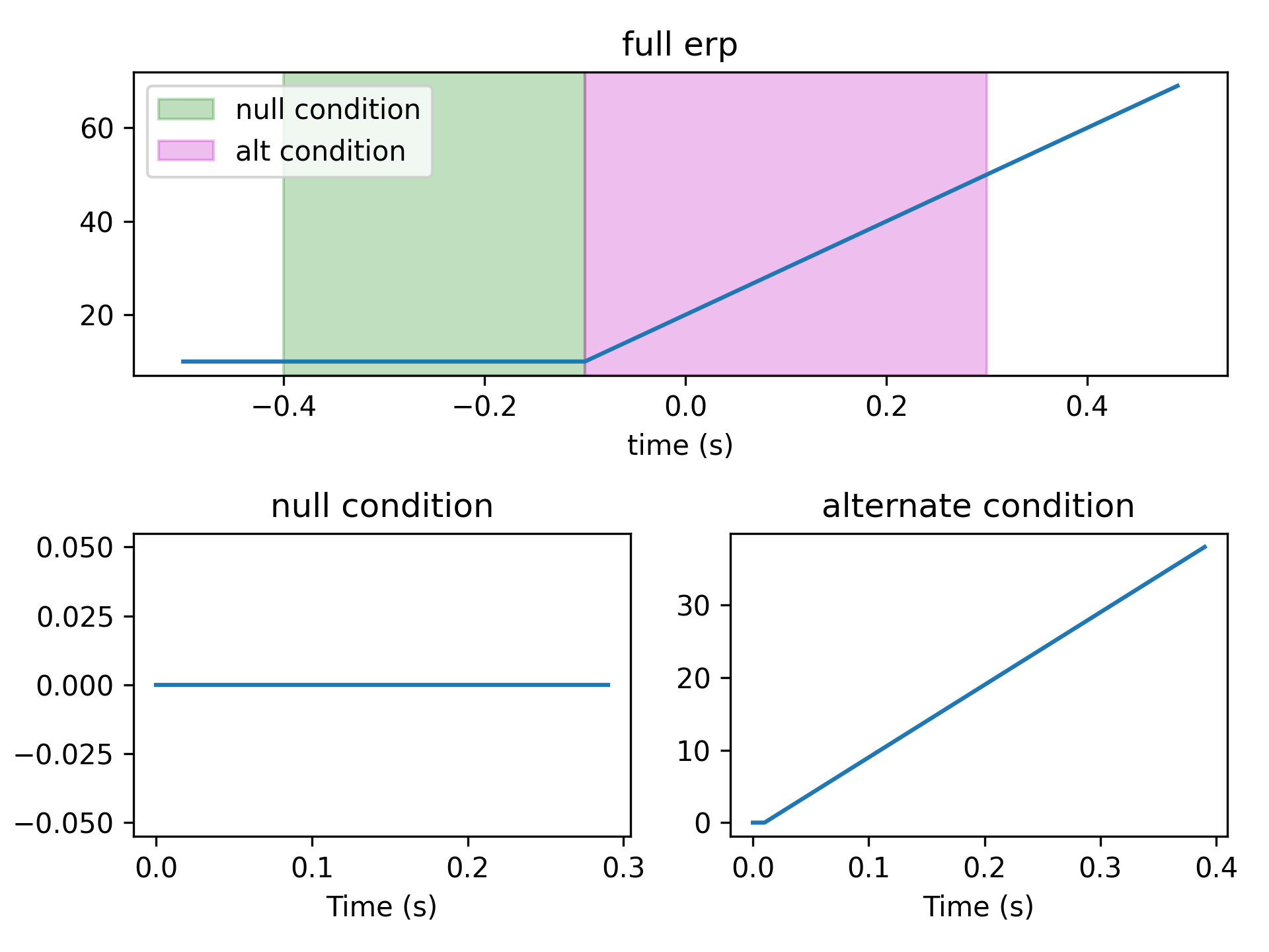
Connectivity

aopy.analysis.connectivity.calc_connectivity_coh(data_altcond_source, data_altcond_probe, n, p, k, samplerate, step, fk=250, pad=2, imaginary=True, average=True)

Calculate the average time-frequency cohereogram between multiple source and probe channels. Iterates through every possible pair (order doesn’t matter) of source and probe channels and calculates the coherence between them. Optionally returns the average across all pairs. This function is called by calc_connectivity_map_coh() to calculate the coherence between a single channel and multiple channels around the stimulation site. No re-referencing is done here, if you want to re-reference the data, do it before calling this function.

Parameters:

• data_altcond_source (nt, n_source, ntrial) – source erp data

• data_altcond_probe (nt, n_probe, ntrial) – probe erp data

• n (float) – window length in seconds

• p (float) – standardized half bandwidth in hz

• k (int) – number of DPSS tapers to use

• fs (float) – sampling rate in Hz.

• step (float) – window step size in seconds.

• fk (float, optional) – frequency range to return in Hz ([0, fk]). Default is fs/2.

• pad (int, optional) – padding factor for the FFT. This should be 1 or a multiple of 2. For nt=500, if pad=1, we pad the FFT to 512 points. If pad=2, we pad the FFT to 1024 points. If pad=4, we pad the FFT to 2024 points. Default is 2.

• imaginary (bool, optional) – if True, compute imaginary coherence.

• average – bool, whether to average the coherence across all pairs

Returns:

tuple containing: | f (n_freq): frequency axis | t (nt): time axis | coh (list of (n_freq,nt)): magnitude squared coherence or imaginary coherence

(0 <= coh <= 1) between the pairs

angle ((list of n_freq,nt)): list of phase difference (in radians) between the pairs (optional output, 0 <= angle <= 2*pi, how much does the probe lead the source)

pair (list of tuples): list of channel pairs

or (freqs, time, coh, angle) tuple**, if average is True

Return type:

tuple

aopy.analysis.connectivity.calc_connectivity_map_coh(erp, samplerate, time_before, time_after, stim_ch_idx, window=None, n=0.06, step=0.03, bw=25, zscore=False, ref=True, parallel=False, verbose=True, imaginary=True, **kwargs)

Map of coherence at every channel to the given stimulation channels. Input ERP data must include at least n seconds before and after events. Coherence is averaged across stimulation channels if multiple are given.

Parameters:

• erp ((nt, nch, ntr) array) – trial-aligned data

• samplerate (float) – sampling rate of the erp

• time_before (float) – time included before events in the erp (in seconds)

• time_after (float) – time included after events in the erp (in seconds)

• stim_ch_idx (list of 0-indexed int) – stimulation channel indices (where you want coherence to be calculated from)

• window (2-tuple, optional) – time window for the coherence calculation in seconds. If None, a single (0, n) window timestep will be used and the step parameter will be ignored. Default None.

• n (float) – window length in seconds for the coherence calculation (default 0.06 s).

• step (float) – window step size in seconds for the coherence calculation (default 0.03 s).

• bw (float) – bandwidth for multitaper filter (default 25).

• zscore (bool) – z-score flag (default False).

• ref (bool) – re-referencing flag (default True).

• parallel (bool or mp.pool.Pool) – whether to use parallel processing. Can optionally be a pool object to use an existing pool. If True, a new pool is created with the number of CPUs available. If False, computation is done serially (the default).

• verbose (bool) – if True, show a progress bar (default True).

• imaginary (bool) – if True, compute imaginary coherence (the default).

Returns:

tuple containing: | freqs (n_freq): frequency axis | time (nt): time axis | coh_all (n_freq, nt, nch): magnitude squared coherence or imaginary coherence

(0 <= coh <= 1) between the pairs at each channel

angle_all (n_freq, nt, nch): phase difference (in radians) between the pairs at each channel

Return type:

tuple

Note

This is not the most efficient way to compute pairwise coherence since we end up repeating the same calculations for each channel multiple times. Maybe a future enhancement. See the implementation in the package spectral_connectivity for a more time-efficient (but memory- inefficient) algorithm.

Examples

Create a grid of channels with mostly noise but two channels have 50 Hz sine waves

grid_size = 3
nch = grid_size**2
T = 1
fs = 1000
nt = int(T*fs)
ntr = 2
time = np.linspace(0,T,nt)
data = np.random.normal(0, 0.1, (nt,nch,ntr)) # start with noise
stim_ch_idx = 0
data[:,stim_ch_idx,0] += np.sin(2*np.pi*50*time) # 50 Hz sine
data[:,stim_ch_idx,1] += np.sin(2*np.pi*50*time)
data[500:,4,0] += np.cos(2*np.pi*50*time[500:]) # 50 Hz cosine in second half of trial
data[500:,4,1] += np.cos(2*np.pi*50*time[500:])

n = 0.25
w = 10
step = 0.25
f, t, coh_all, angle_all = aopy.analysis.connectivity.calc_connectivity_map_coh(data, fs, 0.5, 0.5, [stim_ch_idx],
                                                                        window=(-n, n), n=n, bw=w, step=step, ref=False)

self.assertEqual(coh_all.shape, angle_all.shape)

bands = [(40, 60), (100, 250)]
x, y = np.meshgrid(np.arange(grid_size), np.arange(grid_size))
elec_pos = np.zeros((nch,2))
elec_pos[:,0] = x.reshape(-1)
elec_pos[:,1] = y.reshape(-1)
aopy.visualization.plot_tf_map_grid(f, t, coh_all, bands, elec_pos, clim=(0,1), interp_grid=None,
            cmap='viridis')

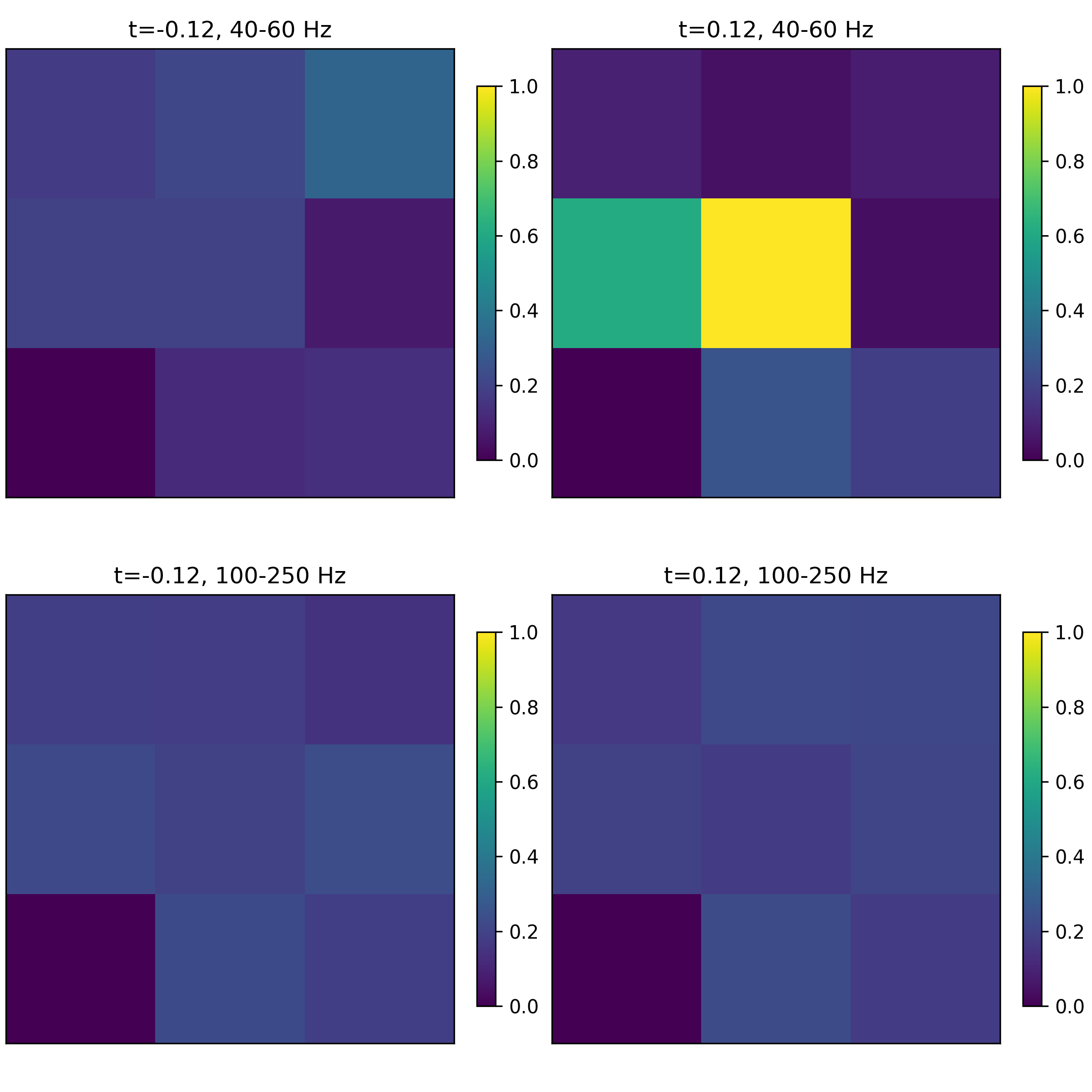
aopy.analysis.connectivity.get_acq_ch_near_stimulation_site(stim_site, stim_layout='Opto32', electrode_layout='ECoG244', dist_thr=1, return_idx=False)

Get acquisition channels near a stimulation site. Use load_chmap() to find the channels for the stimulation and electrode sites.

Note

This function returns channel numbers, which sometimes are 1-indexed. Set the return_idx flag to True to get the channel indices as well.

Parameters:

• stim_site (int) – stimulation site (must match a channel in the stim_layout)

• stim_layout (str) – layout of stimulation sites, e.g. ‘Opto32’. See load_chmap() for options.

• electrode_layout (str) – layout of electrodes, e.g. ‘ECoG244’. See load_chmap() for options.

• dist_thr (float or tuple (min, max), optional) – threshold for distance from stimulation site (in the same units as the electrode layout, typically mm). If a tuple, the distance must be greater than or equal to min and less than max. Default is 1.

• return_idx (bool, optional) – if True, return the channel indices as well. Default is False.

Returns:

np.ndarray, acquisition channels near stimulation site | or (acq_ch, idx) tuple, if return_idx is True

Return type:

acq_ch

aopy.analysis.connectivity.prepare_erp(erp, samplerate, time_before, time_after, window_nullcond, window_altcond, zscore=False, ref=False)

Prepare data for connectivity analysis. Given event-related potentials, extracts a sub-window and normalizes to a baseline null condition. Optionally re-references the data.

Parameters:

• erp ((nt, nch, ntr) array) – trial-aligned data

• samplerate (float) – sampling rate of the erps

• time_before (float) – time before event in the erp (in seconds)

• time_after (float) – time after event in the erp (in seconds)

• window_nullcond ((2,) tuple of float) – desired (start, end) of nullcond (in seconds)

• window_altcond ((2,) tuple of float) – desired (start, end) of altcond (in seconds)

• zscore (bool, optional) – if True, z-score the data. Default is False.

• ref (bool, optional) – if True, re-reference the data. Default is False.

Returns:

alternative condition sub-window of the prepared erp

Return type:

((nt_before_new, nch, ntr) array)