Extract spectral power features

import matplotlib.pyplot as plt
from ipywidgets import interactive, widgets
from tqdm.notebook import tqdm, trange
import os
from datetime import datetime
import numpy as np

import aopy
from aopy.data import db
from aopy.preproc.quality import detect_bad_trials
from aopy.data import get_ts_data_segment, extract_lfp_features, get_extracted_features, get_decoded_states
from aopy.data import tabulate_ts_segments, tabulate_lfp_features, tabulate_feature_data
from aopy.preproc import get_data_segment

/home/aolab/miniconda3/envs/leo-analysis/lib/python3.9/site-packages/one/alf/files.py:10: FutureWarning: `one.alf.files` will be removed in version 3.0. Use `one.alf.path` instead.
  warnings.warn(
/home/aolab/miniconda3/envs/leo-analysis/lib/python3.9/site-packages/statsmodels/tools/_testing.py:19: FutureWarning: pandas.util.testing is deprecated. Use the functions in the public API at pandas.testing instead.
  import pandas.util.testing as tm

Tabulate behavior trials

preproc_dir = '/data/preprocessed'
te_id = 17269
entries = db.lookup_sessions(id=te_id)
decoder = entries[0].get_decoder(decoder_dir='/storage/bmi')

subjects, te_ids, dates = db.list_entry_details(entries)
df = aopy.data.tabulate_behavior_data_center_out(preproc_dir, subjects, te_ids, dates)
display(df[:5])

	subject	te_id	date	event_codes	event_times	reward	penalty	target_idx	target_location	prev_trial_end_time	...	hold_start_time	hold_completed	delay_start_time	delay_completed	go_cue_time	reach_completed	reach_end_time	reward_start_time	penalty_start_time	penalty_event
0	affi	17269	2024-05-03	[16, 65, 239]	[5.84544, 21.85648, 22.86792]	False	True	0	[0.0, 0.0, 0.0]	0.00000	...	NaN	False	NaN	False	NaN	False	NaN	NaN	21.85648	65.0
1	affi	17269	2024-05-03	[16, 80, 18, 32, 82, 48, 239]	[22.88028, 25.82664, 25.84236, 25.85876, 31.81...	True	False	2	[4.9497, 4.9497, 0.0]	22.86792	...	25.82664	True	25.84236	True	25.85876	True	31.81748	31.86540	NaN	NaN
2	affi	17269	2024-05-03	[16, 80, 24, 32, 88, 48, 239]	[34.48108, 42.39212, 42.4078, 42.42248, 44.529...	True	False	8	[-4.9497, 4.9497, 0.0]	32.47432	...	42.39212	True	42.40780	True	42.42248	True	44.52956	44.57456	NaN	NaN
3	affi	17269	2024-05-03	[16, 80, 23, 32, 65, 239]	[47.19256, 47.9506, 47.96468, 47.98, 64.00304,...	False	True	7	[-7.0, -0.0, 0.0]	45.18548	...	47.95060	True	47.96468	True	47.98000	False	NaN	NaN	64.00304	65.0
4	affi	17269	2024-05-03	[16, 80, 23, 32, 87, 48, 239]	[65.02172, 68.63364, 68.65004, 68.6668, 74.456...	True	False	7	[-7.0, -0.0, 0.0]	65.00344	...	68.63364	True	68.65004	True	68.66680	True	74.45600	74.50112	NaN	NaN

5 rows × 23 columns

# Subselect the first 3 rewarded segments
df_sub = df[df['reward']][:3].reset_index()
subjects = df_sub['subject']
te_ids = df_sub['te_id']
dates = df_sub['date']
start_times = df_sub['go_cue_time'].to_numpy()
end_times = df_sub['reach_end_time'].to_numpy()

print(start_times, end_times)

[25.85876 42.42248 68.6668 ] [31.81748 44.52956 74.456  ]

print(decoder.channels)

[ 55  58  60  64  91  97 104 113 211 217 223 227 247 250 252 256]

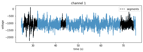
Load neural data

# Plot some neural data from those segments
lfp_segments, samplerate = tabulate_ts_segments(
    preproc_dir, subjects, te_ids, dates, start_times, end_times, channels=decoder.channels-1)

plt.figure(figsize=(8,3))
for idx in range(len(start_times)):
    time = np.arange(len(lfp_segments[idx]))/samplerate + start_times[idx]
    plt.plot(time, lfp_segments[idx][:,1], 'k--', zorder=10)

# Add legends
plt.plot([], [], 'k--', label='segments')
plt.legend()

# Load the full lfp data for comparison
subject = subjects[0]
te_id = te_ids[0]
date = dates[0]

start_time = start_times[0]-1
end_time = end_times[2]+1

lfp_data, samplerate = get_ts_data_segment(
    preproc_dir, subject, te_id, date, start_time, end_time, channels=decoder.channels-1)
time = np.arange(len(lfp_data))/samplerate + start_time

plt.plot(time, lfp_data[:,1], alpha=0.8, label='offline')
plt.xlabel('time (s)')
plt.ylabel('voltage')
plt.title('channel 1')

plt.tight_layout()

Load features using an existing decoder

# Plot the feature segments
features_offline, samplerate_offline = tabulate_lfp_features(
    preproc_dir, subjects, te_ids, dates, start_times, end_times, decoder)
features_online, samplerate_online = tabulate_feature_data(
    preproc_dir, subjects, te_ids, dates, start_times, end_times, decoder)

plt.figure(figsize=(8,3))
for idx in range(len(start_times)):
    time_offline = np.arange(len(features_offline[idx]))/samplerate_offline + start_times[idx]
    time_online = np.arange(len(features_online[idx]))/samplerate_online + start_times[idx]

    plt.plot(time_offline, features_offline[idx][:,1], 'k--', zorder=10)
    plt.plot(time_online, features_online[idx][:,1], 'k--', zorder=10)

# Add legends
plt.plot([], [], 'k--', label='segments')


# Load the full features data for comparison
subject = subjects[0]
te_id = te_ids[0]
date = dates[0]

start_time = start_times[0]-1
end_time = end_times[2]+1

features_offline, samplerate_offline = extract_lfp_features(
    preproc_dir, subject, te_id, date, decoder,
    start_time=start_time, end_time=end_time)
features_online, samplerate_online = get_extracted_features(
    preproc_dir, subject, te_id, date, decoder,
    start_time=start_time, end_time=end_time)
time_offline = np.arange(len(features_offline))/samplerate_offline + start_time
time_online = np.arange(len(features_online))/samplerate_online + start_time

plt.plot(time_offline, features_offline[:,1], alpha=0.8, label='offline')
plt.plot(time_online, features_online[:,1], alpha=0.8, label='online')
plt.xlabel('time (s)')
plt.ylabel('power')
plt.title('readout 1')
plt.legend()

plt.tight_layout()

Note that there is some latency between the offline recorded neural data and the online recorded features.

Thus the online and offline features are slightly different. We try to compensate for this by adding latency to the offline recorded data, as illustrated below. The default latency is 20 ms. Best results using the raw broadband data with no preprocessing (i.e. low-pass filtering) yet applied.

def sweep_latency(e, start_time=10., end_time=20., min_latency=-0.01, max_latency=0.05, step=0.005):
    # Test that extracted features from bci file match the computed features
    subject = e.subject
    te_id = e.id
    date = e.date

    decoder = e.get_decoder(decoder_dir='/storage/bmi')


    features_online, online_samplerate = get_extracted_features(preproc_dir, subject, te_id, date,
                                                                         start_time=start_time, end_time=end_time, decoder=decoder)

    latencies = np.arange(min_latency, max_latency, step)
    corrs = []
    for latency in latencies:
        features_offline, offline_samplerate = extract_lfp_features('/media/moor-data/preprocessed', subject, te_id, date,
                                                                 decoder, start_time=start_time, end_time=end_time,
                                                                 datatype='broadband', latency=latency)
        ch_corr = []
        for ch in range(features_offline.shape[1]):
            corr = np.corrcoef(features_offline[:,ch], features_online[:,ch,0])
            ch_corr.append(corr[0,1])
        corrs.append(ch_corr)

    plt.figure()
    plt.plot(latencies*1000, corrs)
    plt.plot(latencies*1000, np.mean(corrs, axis=1), 'k--')
    plt.xlabel('latency (ms)')
    plt.ylabel('corr coeff')

bci_entries = db.lookup_bmi_sessions(subject='affi', date=('2024-05-03', '2024-05-04'))
print(bci_entries[1].id)
preproc_dir = '/data/preprocessed'
sweep_latency(bci_entries[1])

17269
Downsampling by a factor of 25
Downsampling by a factor of 25
Downsampling by a factor of 25
Downsampling by a factor of 25
Downsampling by a factor of 25
Downsampling by a factor of 25
Downsampling by a factor of 25
Downsampling by a factor of 25
Downsampling by a factor of 25
Downsampling by a factor of 25
Downsampling by a factor of 25
Downsampling by a factor of 25

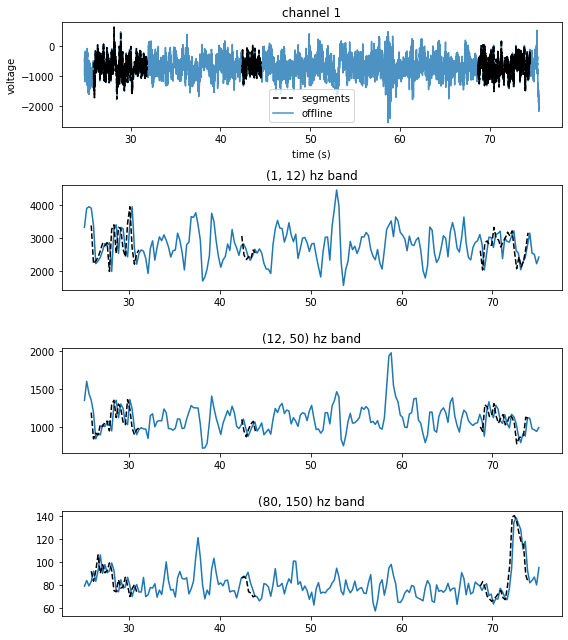
Load arbitrary features from timeseries data

# Fetch some neural data
lfp_segments, samplerate = tabulate_ts_segments(
    preproc_dir, subjects, te_ids, dates, start_times, end_times, channels=[1])

# Extract multiple power bands
bands = [(1,12), (12,50), (80, 150)]
n, p, k = aopy.precondition.convert_taper_parameters(0.5, 25)
step = n/2
fk = 200
features = []
for segment in lfp_segments:
    time, feats = aopy.analysis.get_bandpower_feats(segment, samplerate, bands,
                                                               n=n, p=p, k=k, step=step, fk=fk)
    print(feats.shape)
    features.append(feats)

# Plot
plt.figure(figsize=(8,9))
plt.subplot(4,1,1)
for idx in range(len(start_times)):
    time = np.arange(len(lfp_segments[idx]))/samplerate + start_times[idx]
    plt.plot(time, lfp_segments[idx][:,0], 'k--', zorder=10)

# Add legends
plt.plot([], [], 'k--', label='segments')

for band_idx, band in enumerate(bands):
    plt.subplot(4,1,band_idx+2)
    for idx in range(len(start_times)):
        time = np.arange(features[idx].shape[1])*step + start_times[idx]
        plt.plot(time, features[idx][band_idx,:], 'k--', zorder=10)
    plt.title(f"{bands[band_idx]} hz band")

# Load the full lfp data for comparison
subject = subjects[0]
te_id = te_ids[0]
date = dates[0]

start_time = start_times[0]-1
end_time = end_times[2]+1

lfp_data, samplerate = get_ts_data_segment(
    preproc_dir, subject, te_id, date, start_time, end_time, channels=[1])
time = np.arange(len(lfp_data))/samplerate + start_time

time_feats, feats = aopy.analysis.get_bandpower_feats(lfp_data, samplerate, bands,
                                                           n=n, p=p, k=k, step=step, fk=fk)
time_feats += start_time

plt.subplot(4,1,1)
plt.plot(time, lfp_data[:,0], alpha=0.8, label='offline')
plt.xlabel('time (s)')
plt.ylabel('voltage')
plt.title('channel 1')
plt.legend()

for band_idx, band in enumerate(bands):
    plt.subplot(4,1,band_idx+2)
    plt.plot(time_feats, feats[band_idx,:])


plt.tight_layout()

(3, 22)
(3, 7)
(3, 22)